Extension: realistic source and more detailed geometry

In this brief section, we enhance the source and geometry defined in the Main section, aiming to simulate a more realistic scenario. Working through this extension will give you further practice with building non-trivial geometries, defining realistic beams, and visualizing results in Flair.

Source

Beam

We begin by improving our beam definition. In the Main section, we modeled it as a monoenergetic pencil beam, which doesn't reflect physical reality—real beams always have spatial and energy spread. In FLUKA, these can be defined directly in the BEAM card.

Let’s assume a Gaussian momentum distribution with a FWHM of 5% of the mean momentum (i.e. 1 GeV). We'll also apply a Gaussian spatial distribution with FWHM = 1 cm in both the $x$ and $y$ directions. Under these assumptions, the BEAM card is configured as:

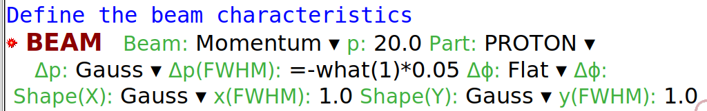
We’ve used Flair's ability to evaluate mathematical expressions, including what(n) references (e.g. what(1) refers to the beam’s mean energy). The minus sign specifies a Gaussian distribution, as described in the manual.

Geometry

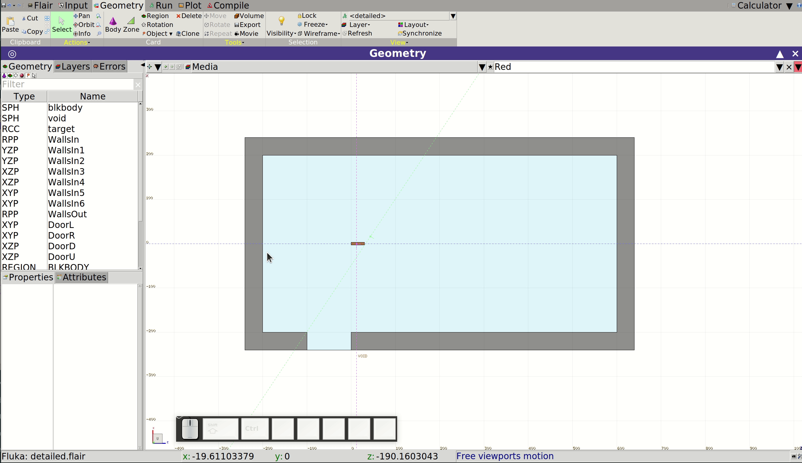
A realistic beam isn't created just in front of the target—it must travel through a beamline, often inside a vacuum pipe. We'll add a cylindrical pipe that enters the irradiation room and position the beam origin inside it using the BEAMPOS card.

First, we need a hole in the wall ahead of the target. Let’s assume:

• Hole radius: 15 cm
• Inner pipe radius: 10 cm
• Pipe wall thickness: 1 cm (aluminum)
• Pipe length inside the room: ~1 m

If you've completed the Main section (and you should!), you already know how to approach this. Try modeling the vacuum pipe yourself before continuing—define the bodies, regions, and assign materials. Focus on structure rather than precise dimensions (these can be adjusted later).

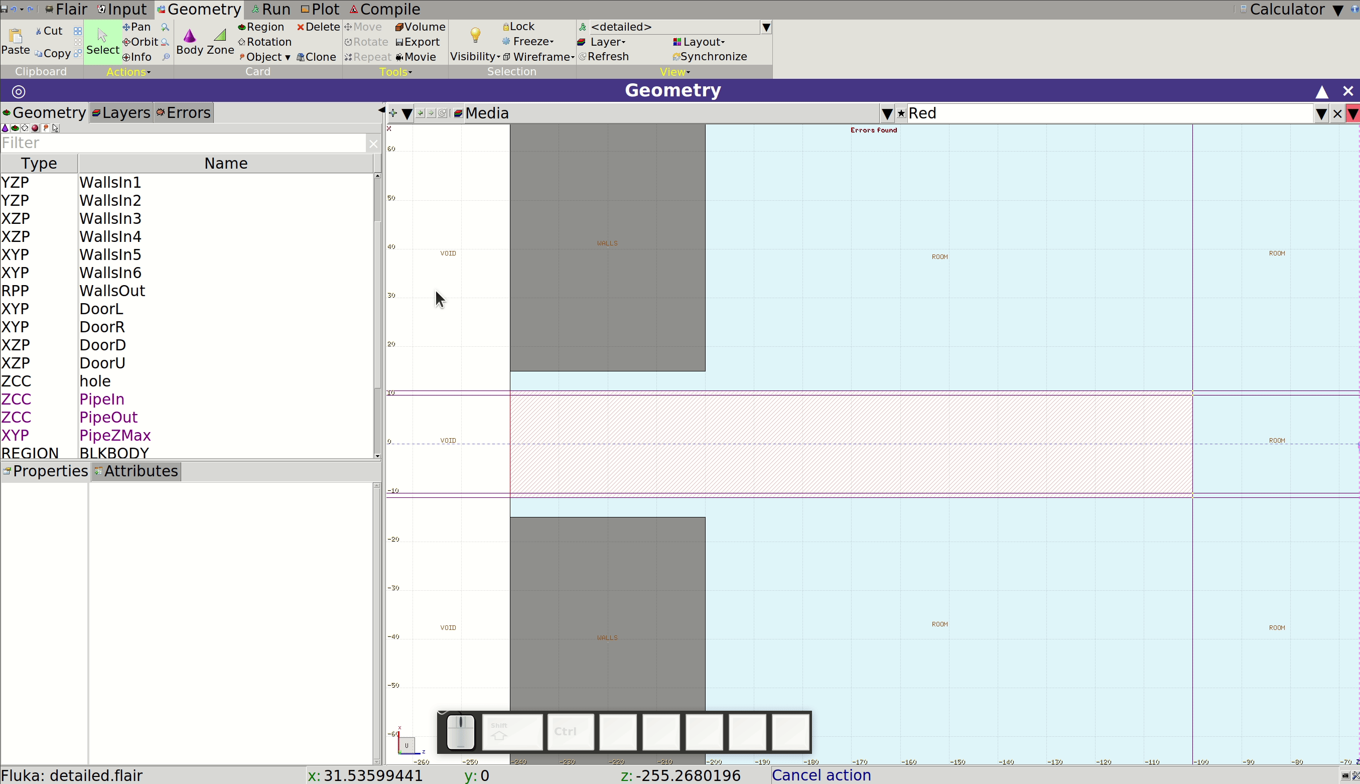
To start, we’ll create the cylinder for the wall hole:

• In the Geometry tab, click Body and choose ZCC.
• Click where the cylinder should be centered
• Adjust its radius and position, then name it (e.g. hole)

Next, subtract this cylinder from the WALLS region:

• Click Zone, then use the pop-up to:
• Select the new cylinder body
• Select the region and the specific zone to modify
• Choose Modify zone under Operation and click on the desired portion to exclude the hole

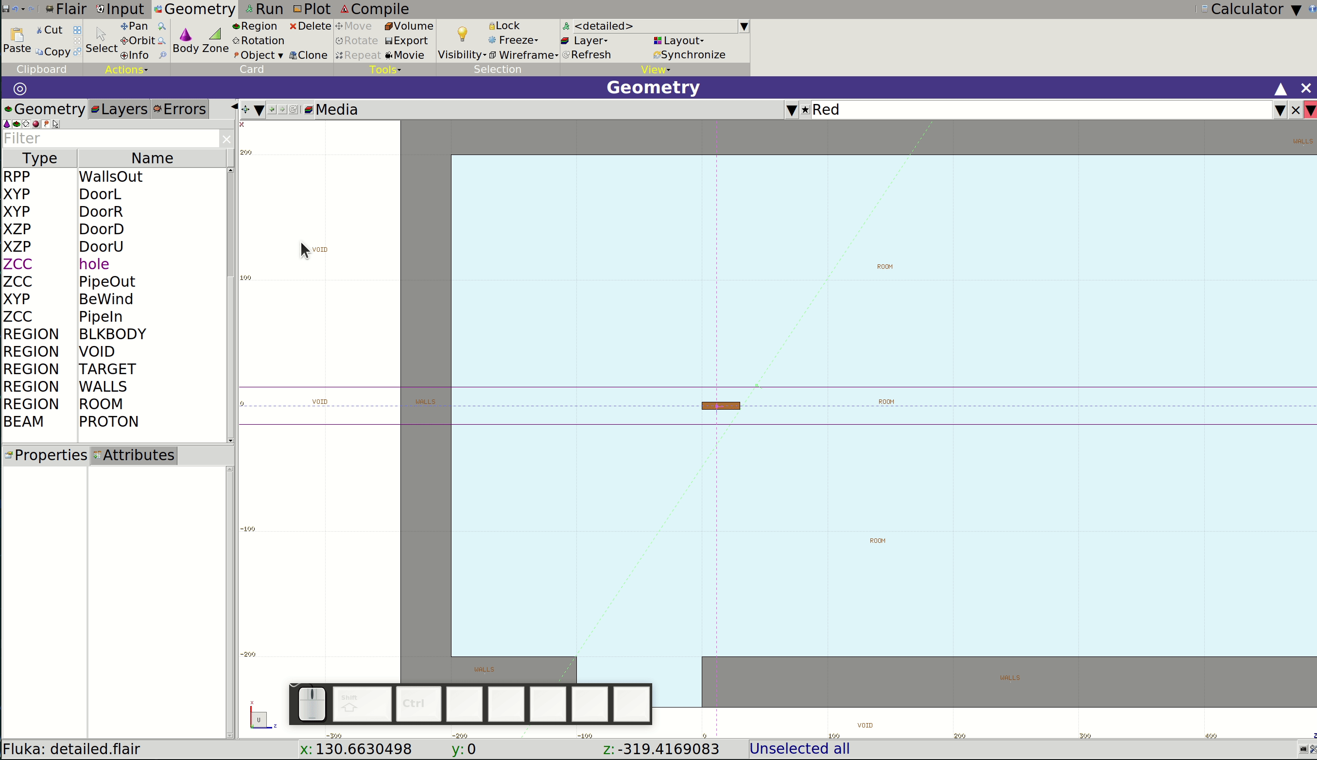
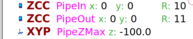
We now define the pipe structure using two infinite cylinders (e.g. PipeIn, PipeOut) and an infinite plane (e.g. PipeZMax) to cap it. The rear boundary will be defined by the existing WallsOut RPP.

Next, modify the ROOM region so that it excludes the pipe and includes the gap between the wall and the pipe. This involves adding two zones to the ROOM region.

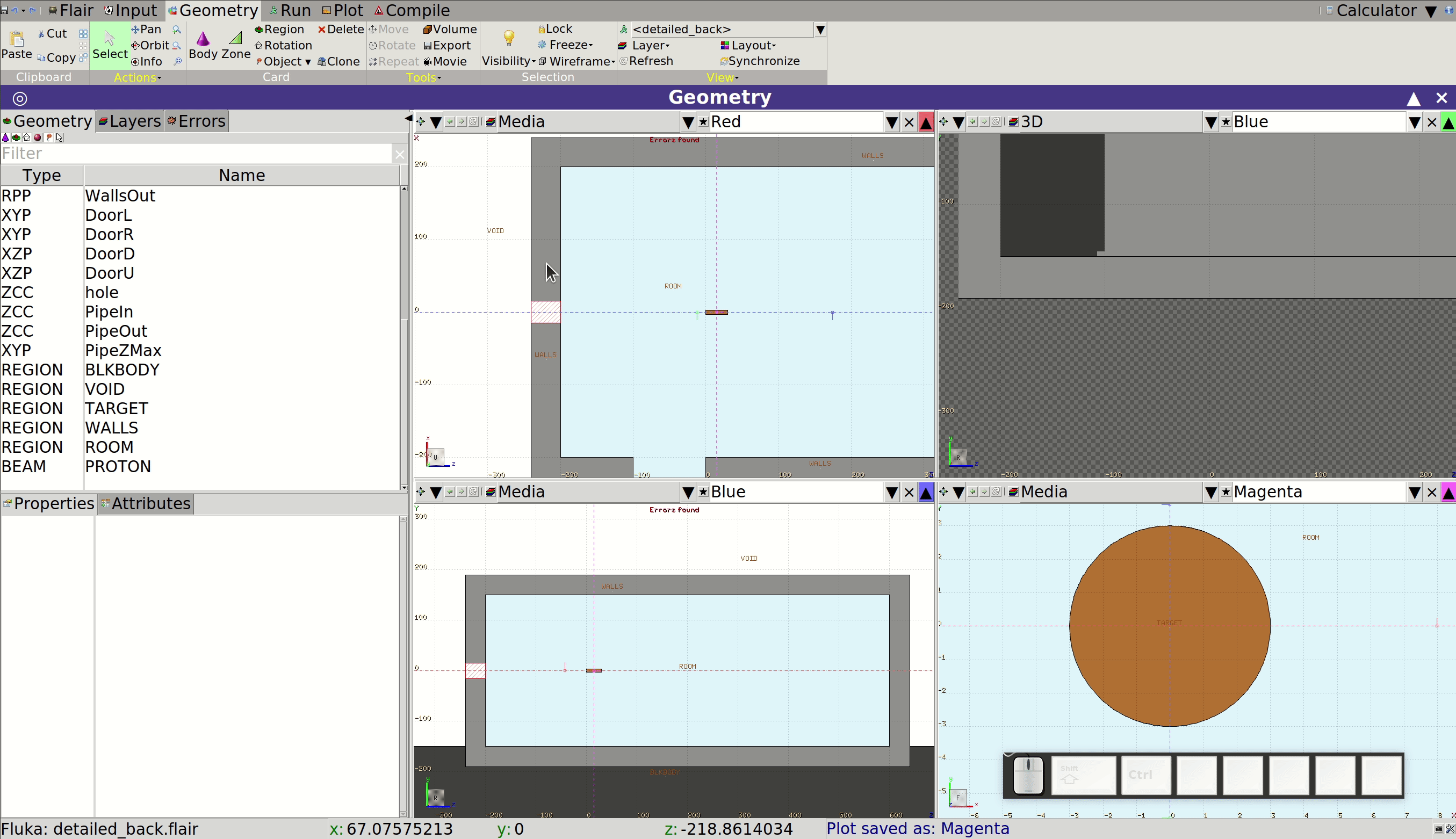
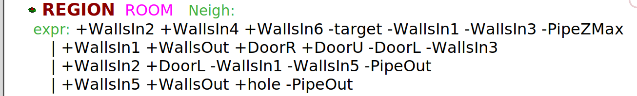
Define the pipe wall region:

• Click Zone
• From the pop-up window, select the bodies that will delimit the new region (here: PipeIn, PipeOut, PipeZMax, WallsOut)
• Choose Add region under Operation
• Place the mouse on top of the portion of space where the new region should go.
• If the shadowed portion of space looks as the new region should, left click to create it. Otherwise the selection of bodies and/or regions was incorrect, restart.
• Name the region (e.g. PIPE) and set its material to ALUMINUM

Repeat the process to define the vacuum region inside the pipe:

Finally, update the proton beam’s origin to $z = -200$ cm using the BEAMPOS card:

Target

Suppose the Cu target includes a water cooling system. This can significantly alter the exiting particle spectra. To model its effect, we’ll add:

• A 1 cm thick water cooling layer around the original target
• A 0.5 cm thick stainless steel cladding around the water layer

You should now be capable of implementing this yourself. The simplest approach is likely to use additional RCC bodies.

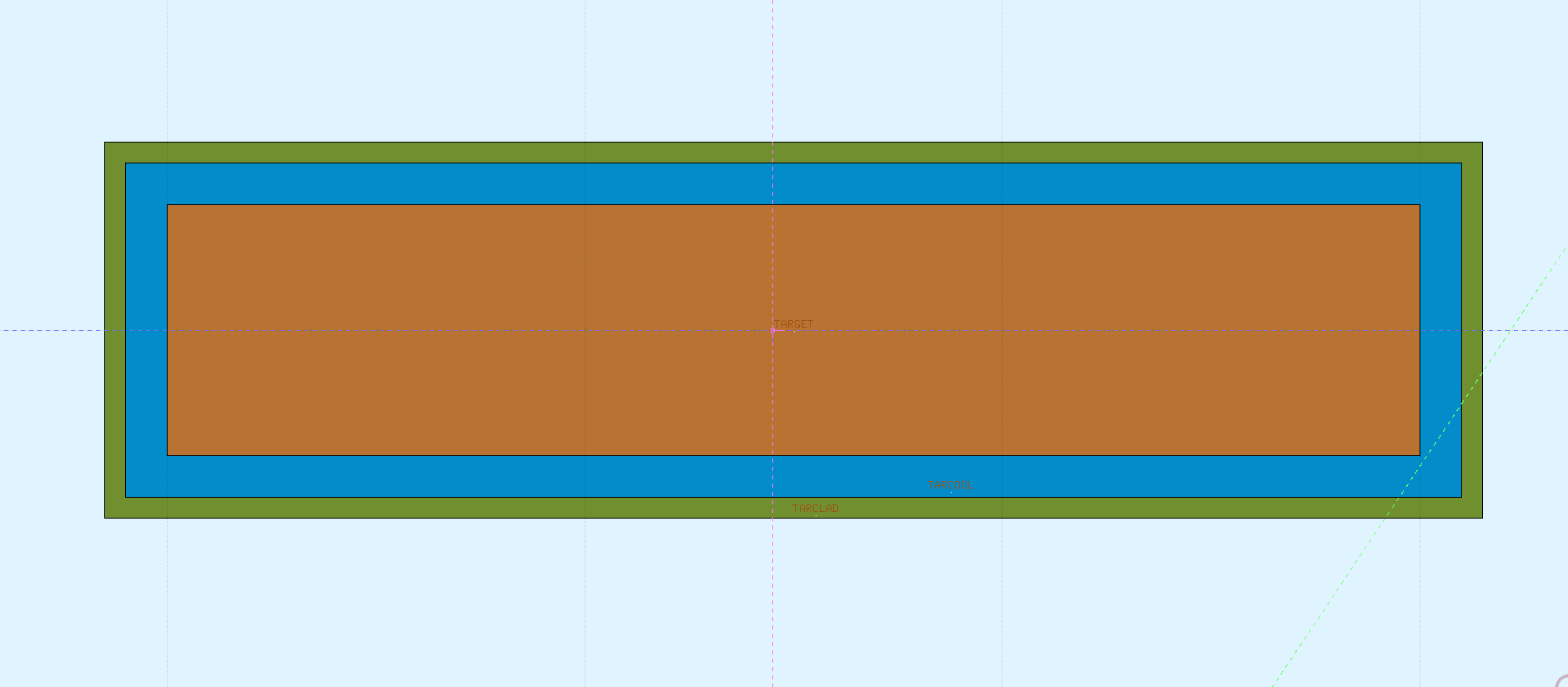
Add the stainless steel material via the Flair material database, just as we did with concrete in the Main section. Any predefined stainless steel will do.

Scoring

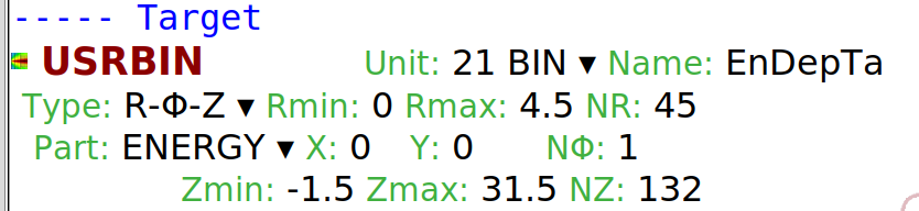
The energy deposition and fluence scorings from Main should be updated to reflect the new target structure. For instance, extend the USRBIN scoring to include the cooling water and cladding:

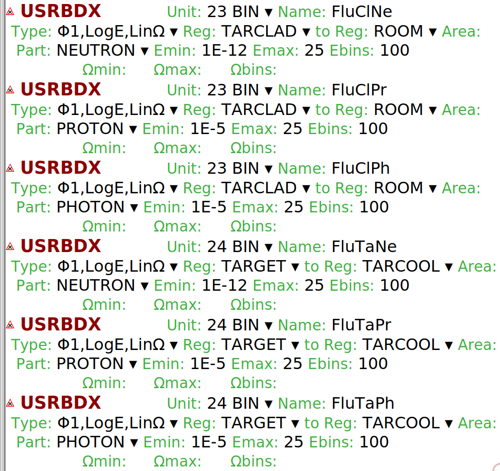
Update the USRBDX scorings to measure particle fluences:

• Between the Cu and water
• Between the cladding and the surrounding room

This allows you to assess the impact of the cooling system.

Given the more complex beam, it’s a good idea to verify its implementation. Such a check is strongly recommended and will save you a lot of time otherwise spent trying to make sense of wrong results. Add scoring to:

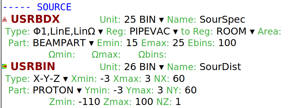
• Check spatial distribution using a Cartesian USRBIN placed inside the vacuum pipe. Score BEAMPART, the fluence of primary particles. We are interested in the $x$ and $y$ directions, so only 1 bin is necessary along $z$.
• Check energy spectrum using a USRBDX at the boundary between the pipe vacuum and room air

The resulting scorings should look like the followings:

Choose a binning fine enough to reveal structure but coarse enough to accumulate meaningful statistics.
Feel free to add more scorings if you are interested in other quantities and/or other locations!

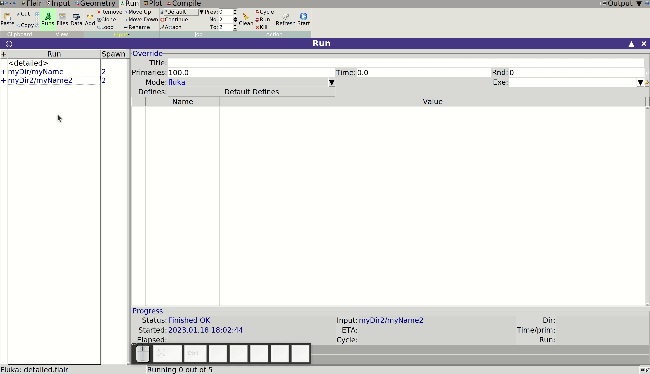
Run and process

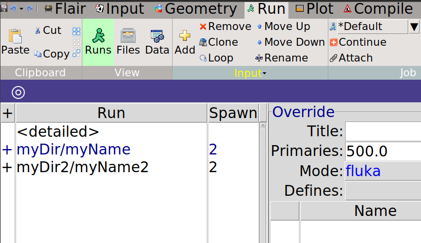
Running the simulation follows the same process described in Main. You can create multiple Runs with different names or directories to avoid overwriting results:

If not all your detectors appear under the Data tab, click the Scan button to refresh the list based on your input file:

Results

Beam

We begin by validating our updated beam configuration. In the Plot tab:
- Click Add, then choose USRBIN
- (Optional) Rename the plot with a descriptive title
- Click the folder icon to select the appropriate result file
- Under Title, enable the grid and set the aspect to 1 to maintain a 1:1 ratio between the $x$ and $y$ axes
- Click Plot

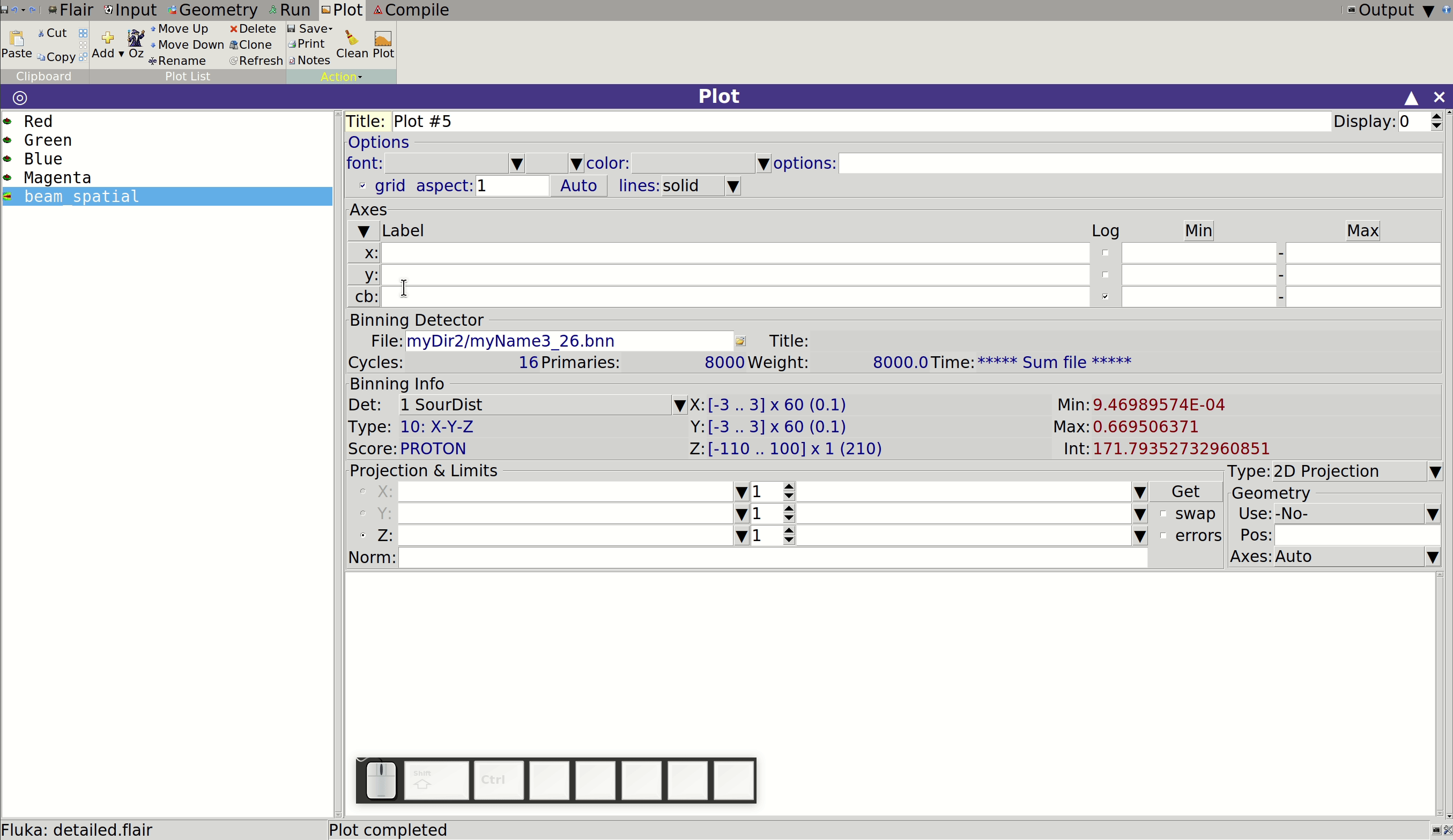
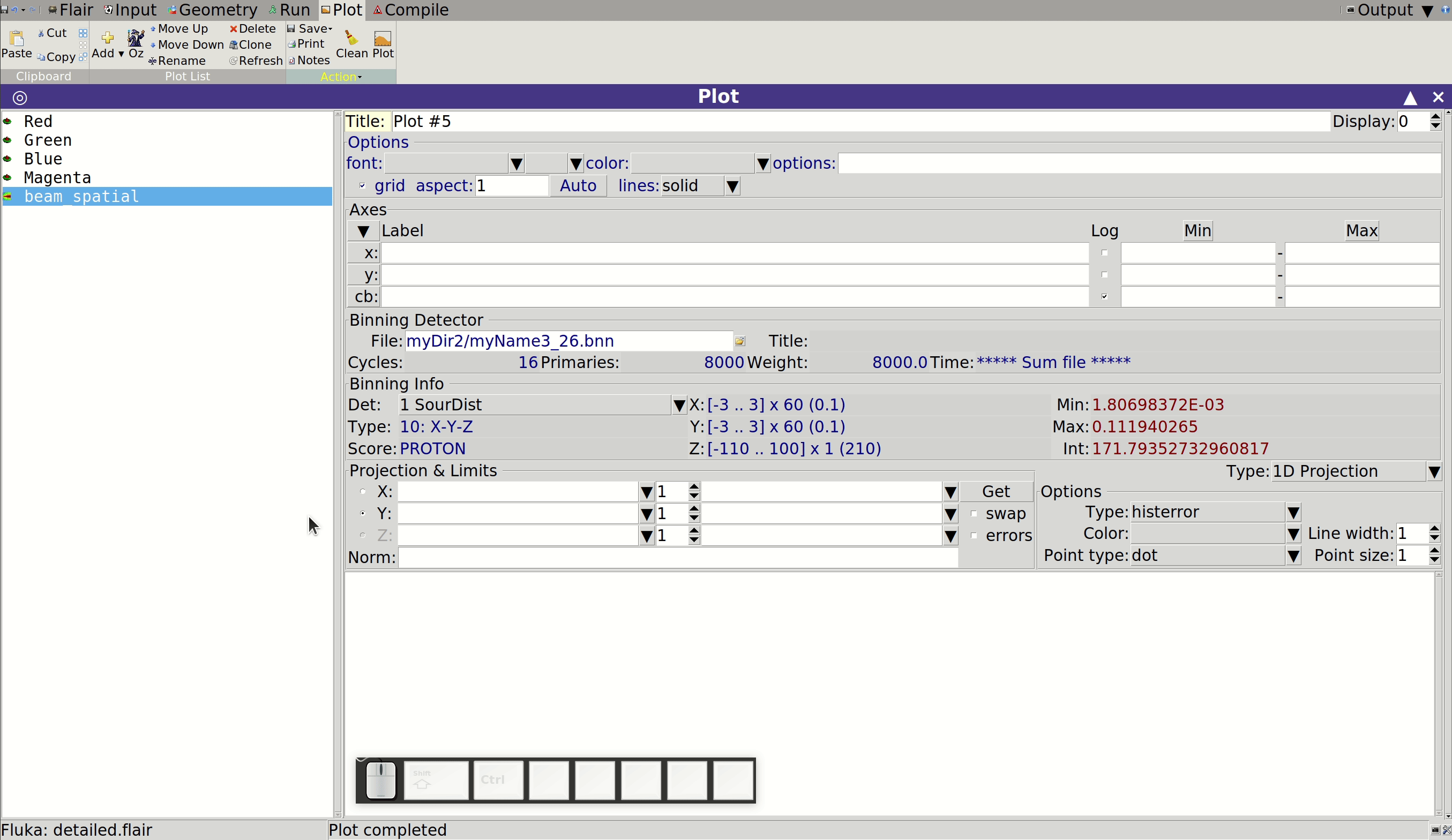
If you encounter a file error, follow Flair's on-screen suggestion (usually to reprocess or rescan). Now, observe the 2D distribution. Does it resemble a Gaussian centered on the beam axis, with the expected spread in $x$ and $y$?

To examine this more closely, switch to 1D projections:
- Set Type to 1D Projection
- Enable projection along $x$, $y$, or both by ticking the appropriate boxes

If statistics are insufficient to assess the beam profile, consider increasing the number of primary particles, cycles, or spawns in your simulation.

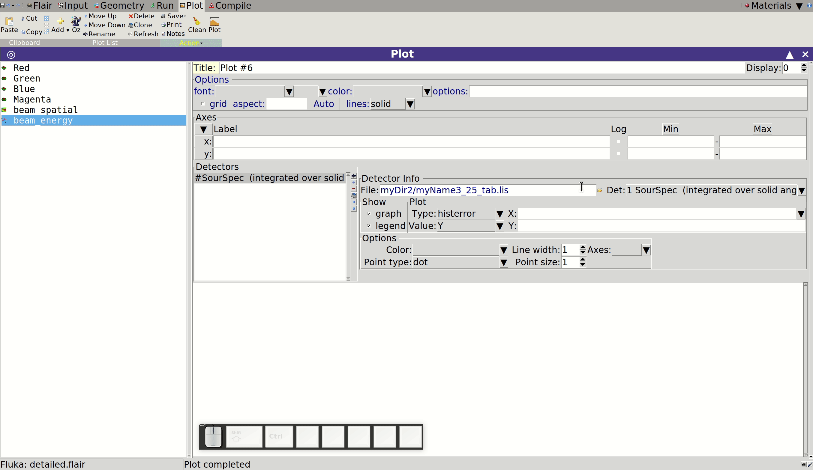
Next, let’s examine the energy spectrum of the beam using the USRBDX scoring defined at the pipe-room boundary. Create a USR-1D plot and select the processed results file:

Now consider: does the spectrum match your expectations? The beam was defined with a mean momentum of 20 GeV/c, but the scoring outputs kinetic energy. To verify the conversion, go to the Calculator tab:
- Under Functions, choose Physics → Momentum to Energy
- Enter the momentum (20 GeV/c) and select Proton mass from the Particles menu

You should find the mean energy around 19 GeV. Does your scoring reflect this? Also, does the spread correspond to the 1 GeV FWHM we specified?

Target

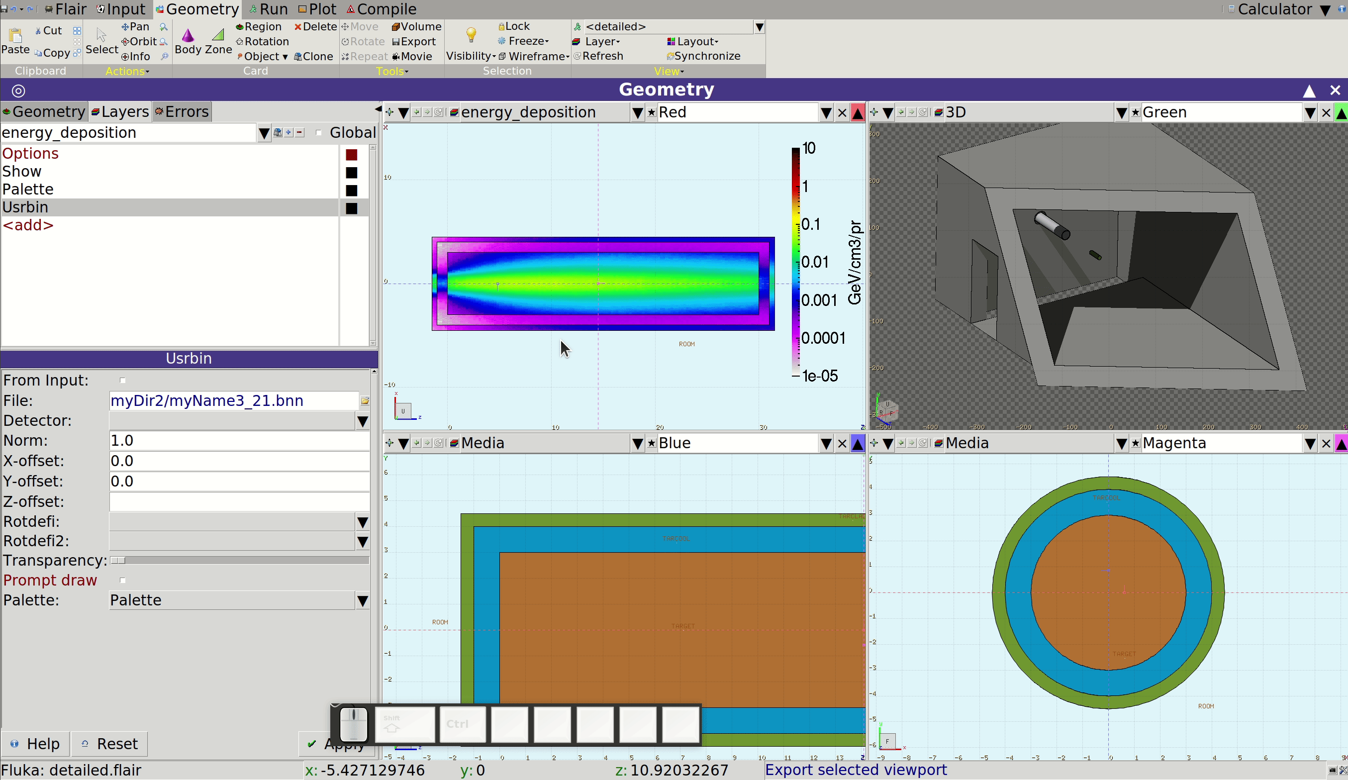
Now let’s inspect the energy deposition in our modified target. Visualize the USRBIN results in the Geometry tab using a dedicated layer:
- Navigate to the appropriate viewport
- Use the Export button (top of the window, near Visibility) to save the view
- In the pop-up window:
* Select the relevant viewport
* Set Type to Notes
* Choose image size manually or via template
* Click Export and wait for confirmation

To compare with the result from the Main section, export that plot as well using a separate geometry layer. This prevents overwriting the first image and enables direct comparison:

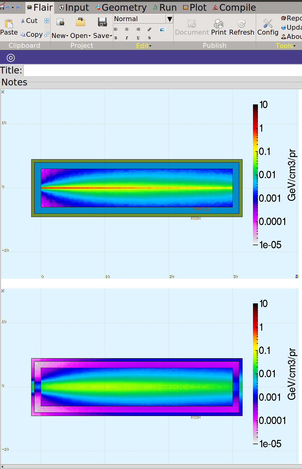
You’ll likely observe a broader energy deposition pattern due to the beam spread, as well as noticeable transitions between copper, water, and steel. These transitions should align with the material properties and their expected stopping power.

Lastly, examine the new fluence distributions. Plot the results of both USRBDX scorings:
- One at the boundary between copper and cooling water
- Another at the boundary between the cladding and surrounding air

Use distinct colors for clarity:

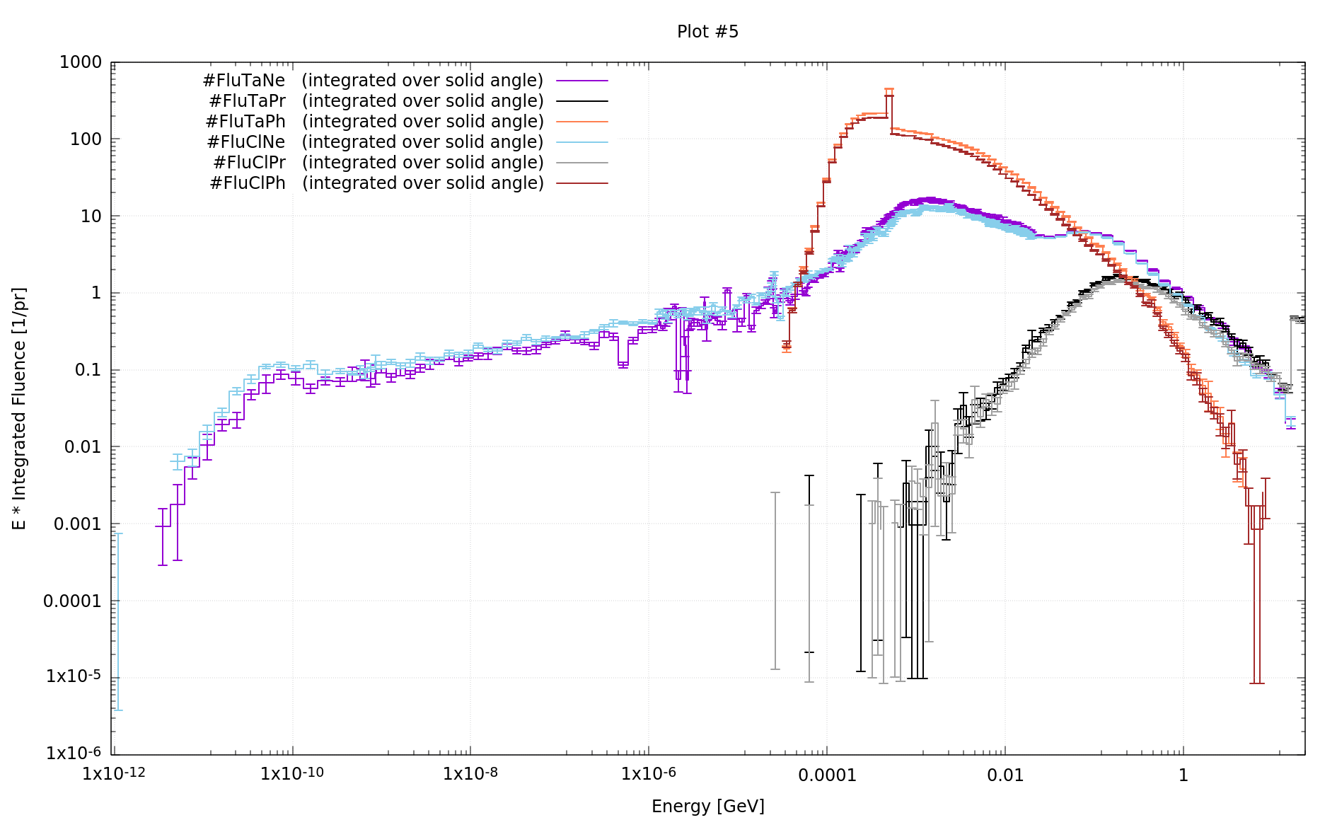
These plots were produced using 8000 primary particles. To evaluate the integrated fluence (total particles crossing a surface), do not apply surface normalization. This makes it easier to compare the cumulative effect of different layers.

From the results, we observe:
- A general reduction in fluence after adding water and steel layers
- Photon fluence drops by ~15–20%
- Proton fluence decreases by up to 30–35% at certain energies
- Thermal neutron fluence increases by roughly 40%
- Fast neutrons (in the MeV range) show a reduction of up to 30%

Congratulations! If you've successfully followed this extension, you're now comfortable with modeling realistic FLUKA geometries and setups. You've gained hands-on experience with beam design, scoring, simulation, and results interpretation. Hopefully, you’ve also uncovered more of Flair’s helpful features. If you have any questions, visit us on the FLUKA forum.