In this example, we will create a toy model of a mixed-field irradiation facility to put into practice many of the concepts explained in the beginner's guide. We will begin with a first approximation that allows us to obtain rough estimates for a few quantities of interest. More specific calculations will be tackled in extensions to this example.

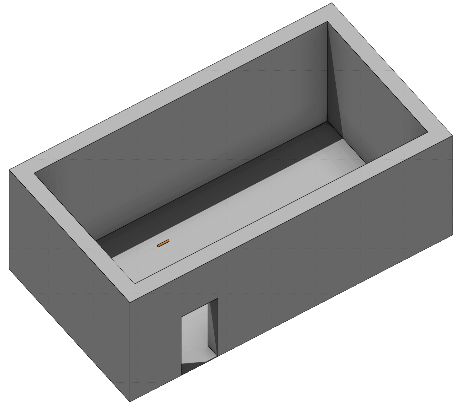
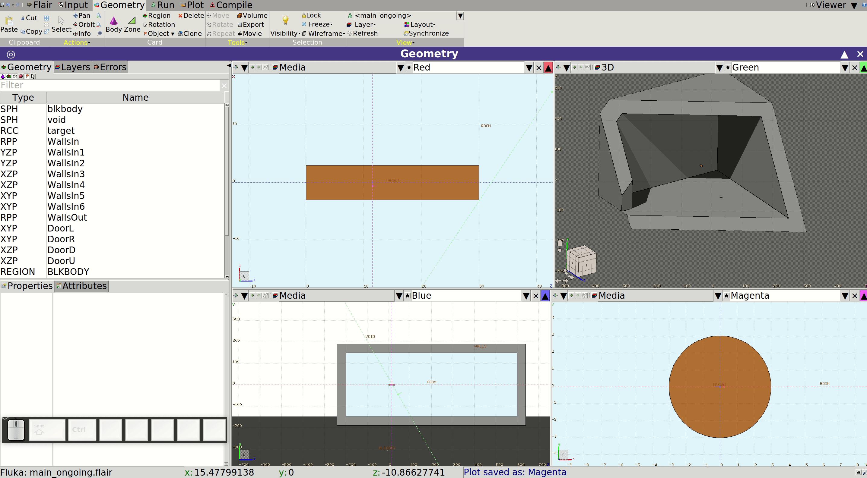
The first thing we need is a radiation source. We will consider a pencil proton beam with a momentum of 20 GeV/c. The beam will strike a cylindrical copper (Cu) target, generating a mixed-field radiation environment. Naturally, an irradiation facility requires shielding, so we’ll add walls to our model. The resulting geometry should resemble the one below (note that the ceiling has been removed for illustrative purposes):

Our goal is to obtain initial estimates for several quantities of interest:
- particle fluences on the surface of the target
- energy deposition within the target
- dose-equivalent in the room.

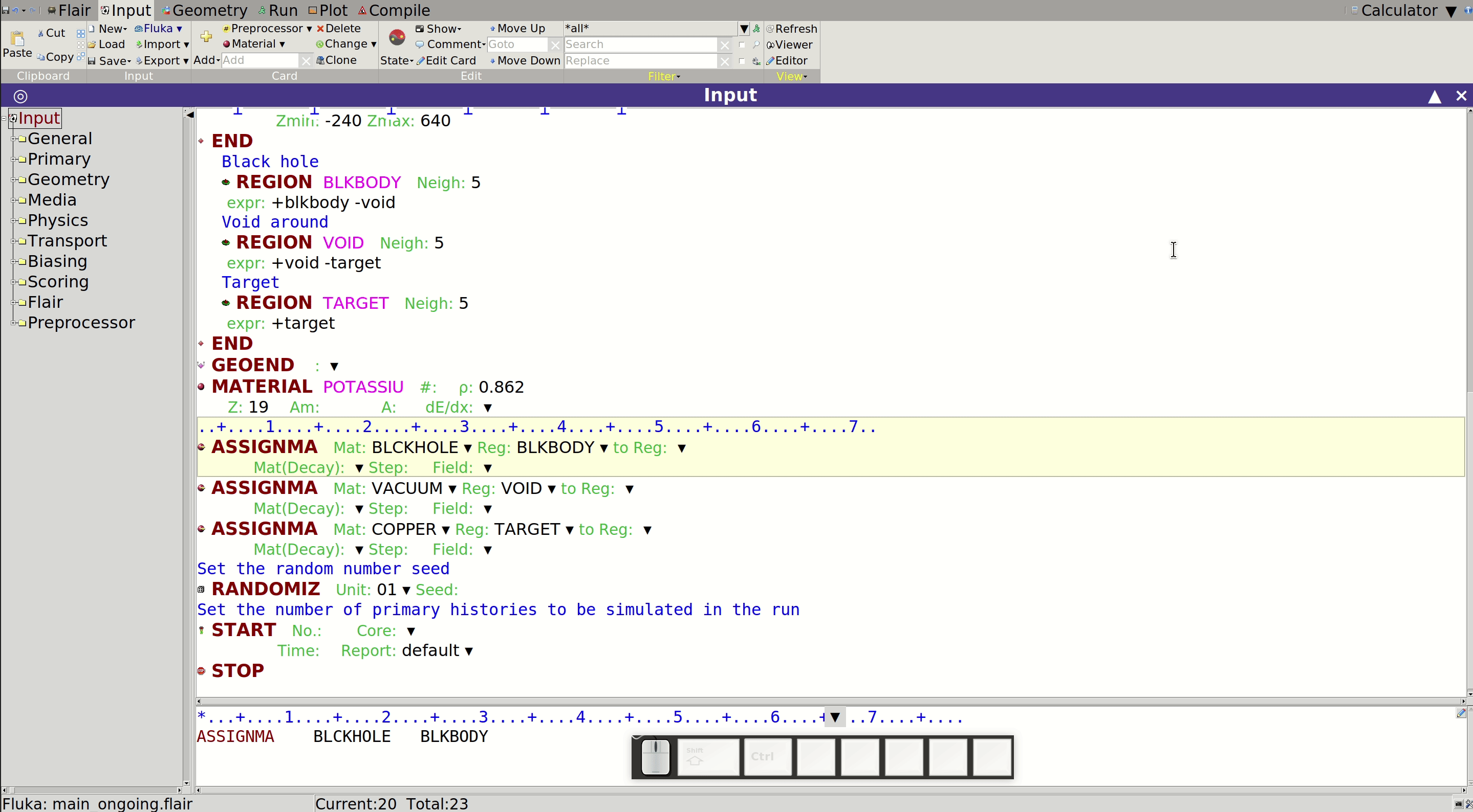
Input file

In this subsection, we will build the FLUKA input file step-by-step using Flair.

Basic input

We begin by loading a basic input file template in Flair. This helps ensure we include all essential sections and maintain a logical structure.
To load the template such example:
- Open Flair
- Navigate to the Input tab
- Click the New button (top left corner)
- Select basic in the dropdown menu

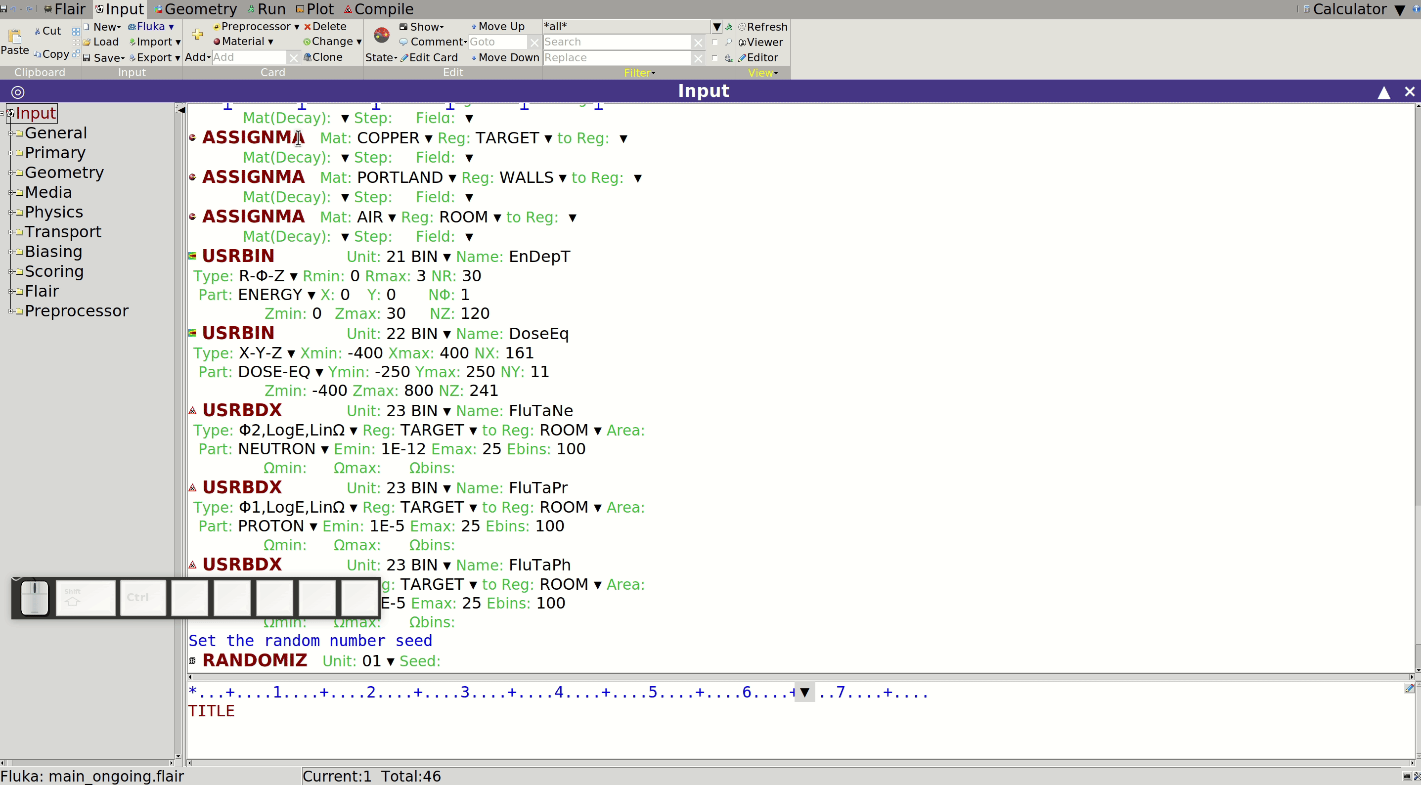
Take a moment to inspect the input file and visualize the geometry in the Input and Geometry tabs. Note that no specific scoring is requested, and no materials are defined. That’s because the materials used are predefined in FLUKA.

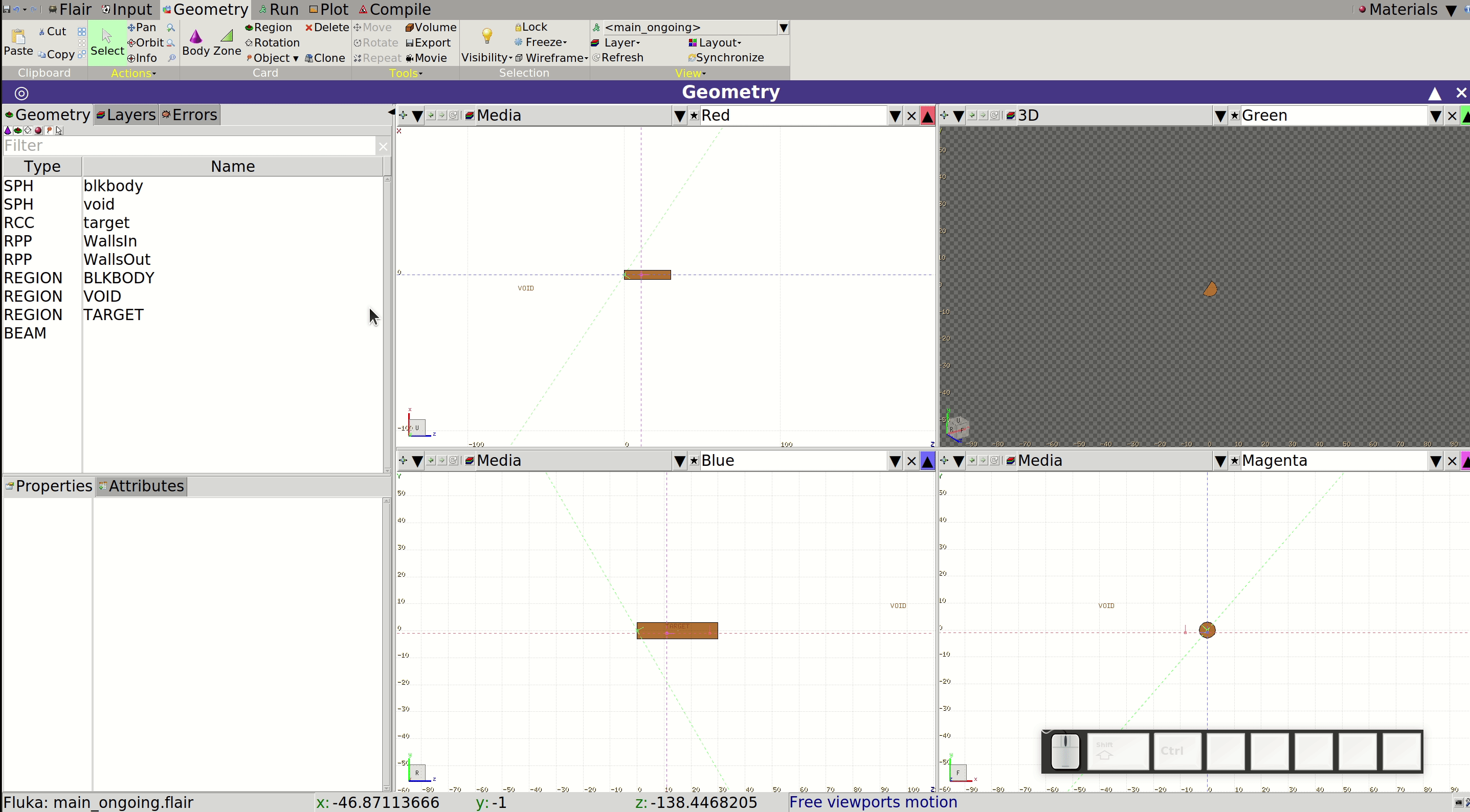
Geometry

The geometry can be divided into three main parts: the target, the walls, and the air inside the room. Additionally, we’ll add a ground surface to improve visualization. Everything else should be filled with void to ensure no CPU time is wasted simulating interactions in areas outside the facility.

As we’ve seen earlier, Flair allows us to edit the geometry either directly in the input file (Input tab) or via the visual geometry editor (Geometry tab). Both approaches work in most cases, though the geometry editor is often preferred when constructing regions, as its visual interface helps avoid errors.

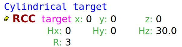
Let’s start with the copper target. We can modify the existing target defined in the basic template. Select the RCC body named target, and set its height ($H_z$) to 30 cm and its radius ($R$) to 3 cm. This can be done in either the Input or Geometry tab. Leaving its position unchanged places it at the origin of the coordinate system.

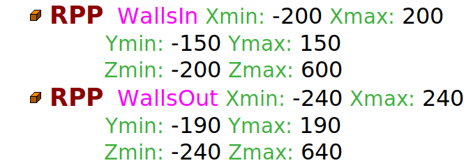
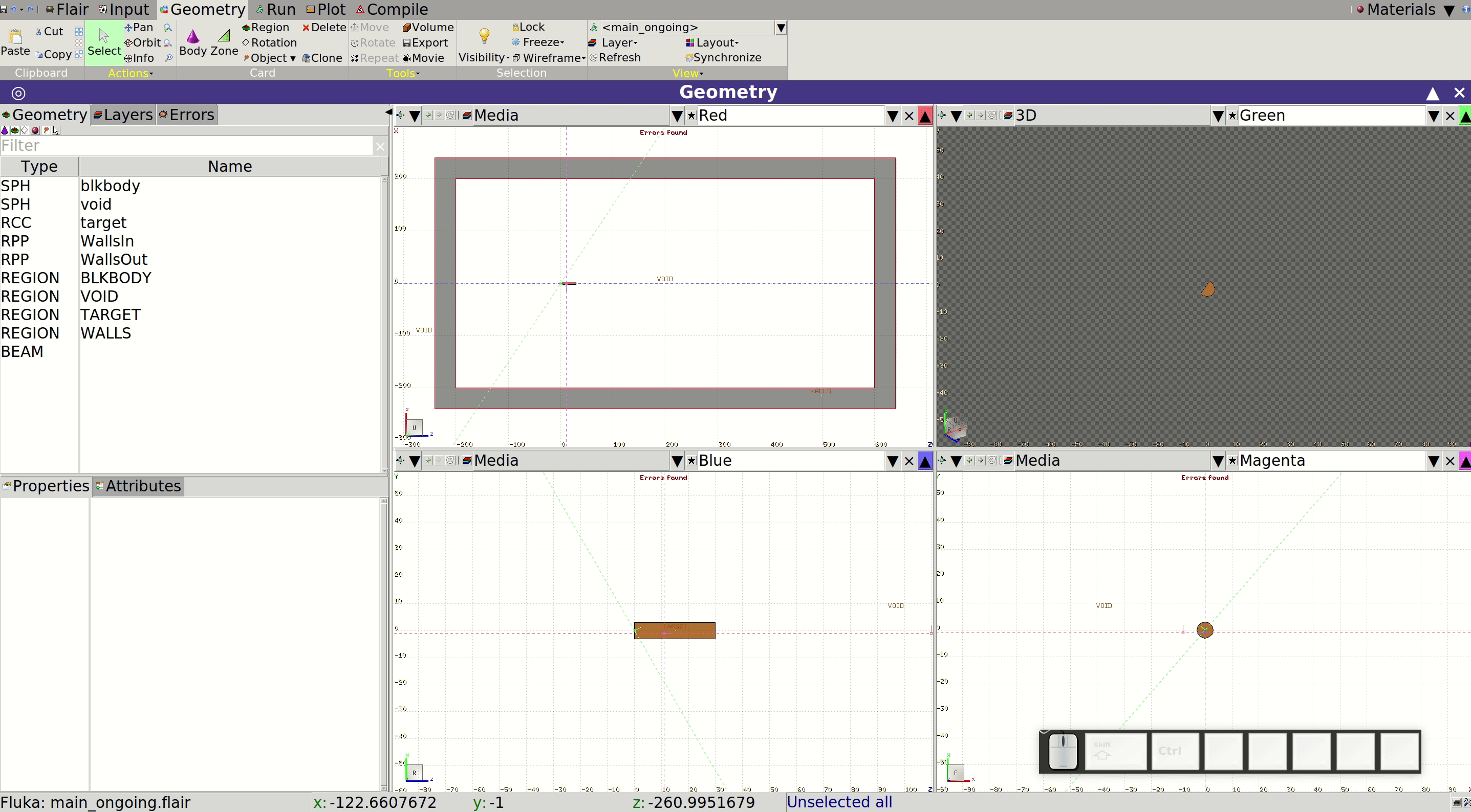
Next, let’s tackle the room walls. A convenient approach is to create two RPP bodies, one inside the other, to define all walls at once. Assume the room has dimensions of 400 $\times$ 300 $\times$ 800 cm³ ($xyz$), and the wall thickness is 40 cm. We’ll place the target in the middle of the room along the $x$ and $y$ axes, and 2 m from the nearest wall along the $z$ axis. This way, with the beam entering in the positive $z$ direction, we leave space downstream for future components. The resulting RPPs are:

The walls will be made of concrete. Until we obtain detailed information about their chemical composition, we will use the predefined "Concrete portland" material available in the Flair database. This may not match the actual wall composition and could impact our results. To add the material:

• Go to the Materials tab (you may need to click the black down arrow at the top right of Flair to find it)
• Search for "concrete" in the Search field
• Select Concrete portland
• Click To input (top left corner of Flair)
• In the pop-up, select Only MATERIAL card to add the material and compound cards to your input

Return to the Input tab to confirm the cards were added.

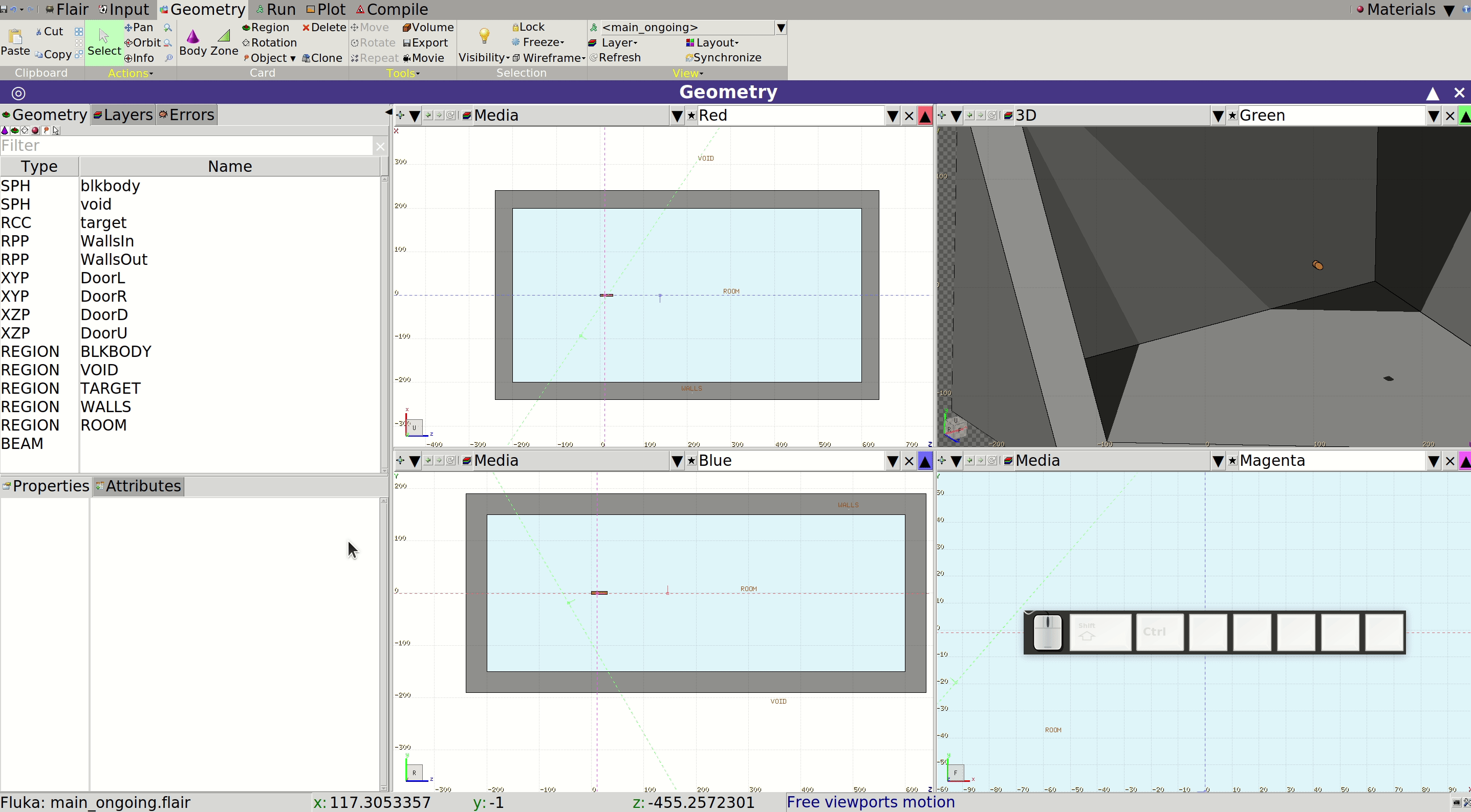
Next, we define the Region representing the walls. Open the Geometry tab to use Flair’s geometry editor. You should see the Cu target.

We’ll focus on the red viewport, which shows a cross-section along the $xz$ plane at a given $y$ height (each viewport can be identified by the colour of its top-right button, which displays an upward arrow). The wall region comprises the space between the two RPPs. On the left side of the Flair window, under the Geometry sub-tab, you’ll find the RPPs’ names. Select them to visualize their outlines. If they’re not visible, zoom out.

To create the region:
- Ensure only both RPPs are selected
- Click Zone (top left of Flair)
- Move the cursor to the space between the RPPs. When the space is shadowed, left-click
- A new region named REG1 is created. Rename it to WALLS in the bottom-left properties panel
- Set its material to PORTLAND (from earlier)

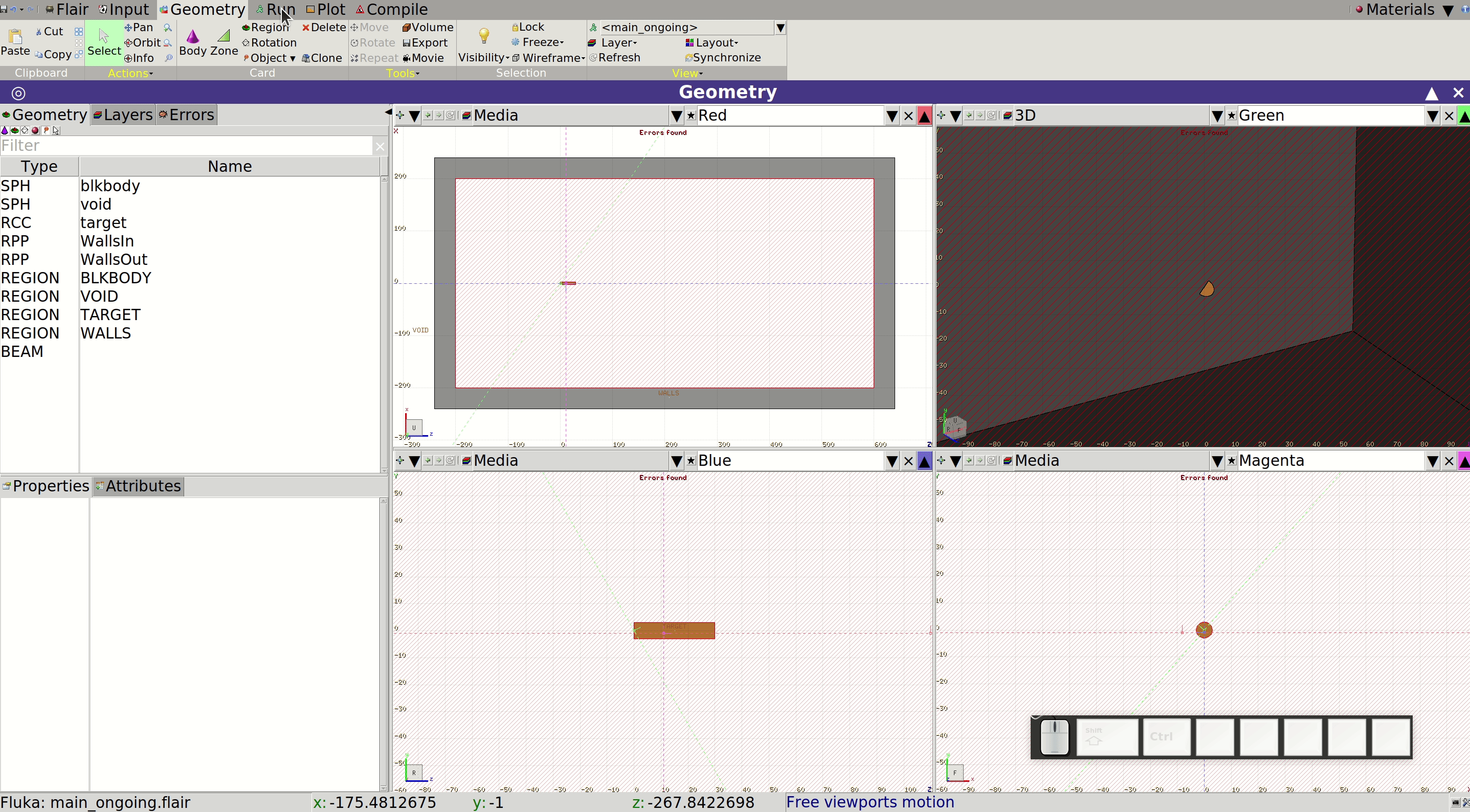
As you may have noticed, the space between the walls' RPPs is now part of two regions: WALLS and VOID. Take some time to explore the visual feedback to confirm this. For instance, select different regions and observe how they are highlighted in the viewports. Clicking on the wall region in any viewport should highlight both region names in the list on the left, indicating that the selected point belongs to both. Note also the Error found flag at the top of the viewport. In FLUKA, each point in space must belong to only one region, so we need to resolve this overlap.

We want everything outside the walls to be part of the VOID region. To fix the overlap, we need to update the VOID region definition to exclude the space within the outermost wall RPP. In the geometry editor:

• Select the zone you want to modify (not just the region)
• While the zone is selected, select the relevant bodies that define the new expression
• Click on Zone (top left)
• Hover the cursor over the space to be included in the updated zone and left-click when it's correctly highlighted

You can select zones, bodies, or regions either from the list on the left or directly in the viewports. A pop-up window will guide you through the process after clicking Zone.

After making this change, there will be a remaining volume—namely, the room itself—that doesn’t belong to any region. Since every space that a particle might traverse must belong to a region, we must define this missing region.

Proceed similarly to how you defined the WALLS region. In this case, the material should be AIR, which is predefined in FLUKA:

• Select the appropriate bodies (e.g. WallsIn and target)
• Click Zone at the top left
• Left-click when the correct volume is highlighted
• Rename the new region to ROOM and assign the material AIR

We now have a valid, albeit simple, geometry that could already yield useful simulation results. However, let’s enhance it with an additional feature: a door.
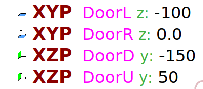
A door is essentially a rectangular hole in the wall. A clean way to create one is by using four planes to carve it out—two XYP and two XZP planes. The door will measure 200 × 100 cm² ($y*z$), located in the right-side wall from the beam’s perspective (i.e., the wall with the lower $x$ coordinate). For instance:

• $x_0 = -100$, $x_1 = x_0 + 100$
• $y_0 = -150$, $y_1 = y_0 + 200$

Before altering the WALLS region, let’s attempt to add a new zone to the ROOM region to include the door threshold. This will help uncover a potential issue. To do so:

• Select the ROOM region (not a zone)
• Select the door-defining bodies and the relevant wall RPPs
• Click Zone and define the new volume

You'll likely observe that two doors are created. This happens because of how the walls were originally described—as the space between two RPPs, which lacks directionality (e.g. left vs. right). Ideally, we would use infinite planes for the WALLS definition, but we chose RPPs for convenience.

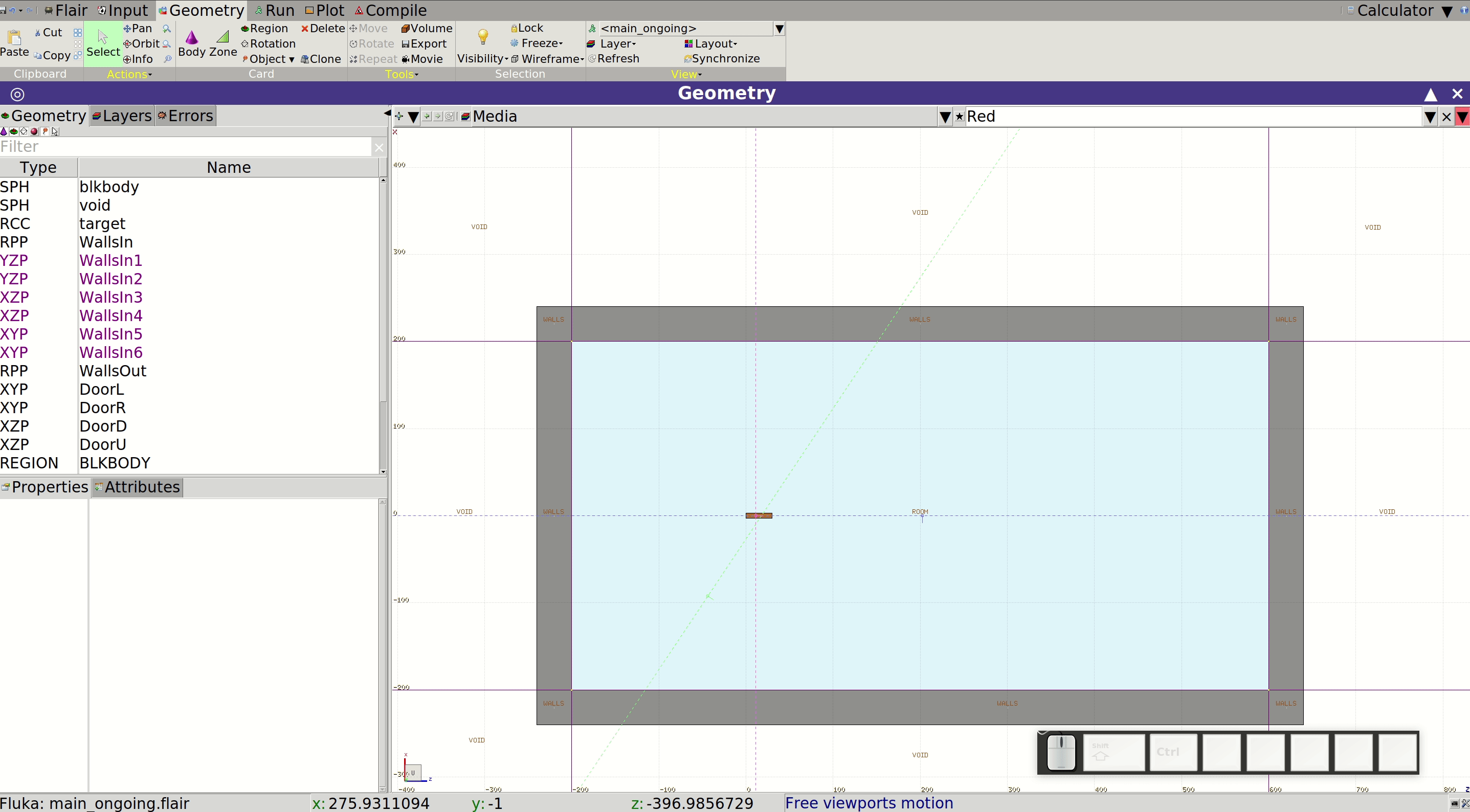
Fortunately, Flair allows you to convert RPPs into sets of infinite planes and automatically updates region definitions accordingly. To fix this:

• Select the inner RPP
• Click Expand (middle-right area)

Verify that the conversion occurred. If parentheses are now part of the region expressions, click Expand again to remove them (recommended for performance reasons). You may also use Optimize to clean up any redundant zones.

Now try adding the door threshold to the ROOM region again:

• Use the same bodies as before (four planes + walls' RPP + inner limit plane)

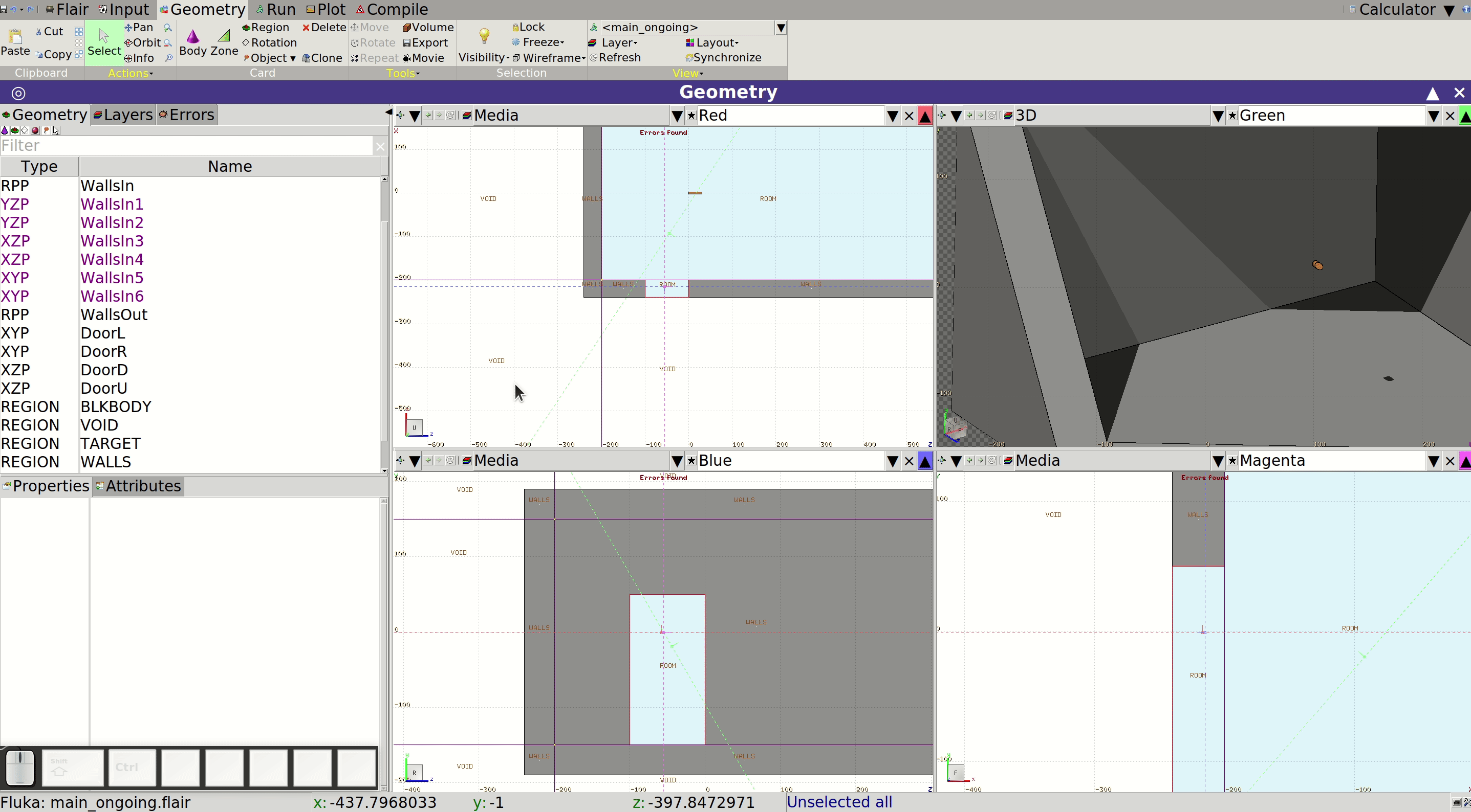
This volume now belongs to both ROOM and WALLS. You must remove it from the WALLS definition. To make this clearer, focus on the red and blue viewports (top and side views respectively). Center the viewports on the door by clicking over the area and pressing c on your keyboard.

You may notice that two XZP planes at $y = -150$ cm are being used—one for the room floor and one for the door base. It’s best to use a single shared plane here to prevent potential numerical issues. Replace the duplicate plane in the ROOM region with the one used in WALLS, then delete the redundant one.

Now we can modify the WALLS region to exclude the door threshold area. There are two options:

• Manually replace the affected zone with several new ones
• Reuse the door threshold zone expression from ROOM and subtract it from WALLS using parentheses, then click Expand and Optimize

Zone overlaps (within the same region) are acceptable and even beneficial for performance in FLUKA, unlike region overlaps, which must be avoided.
Lastly, we’ll extend the BLKBODY region to simulate the ground. This region uses BLCKHOLE as the material, which absorbs all particles that enter. To do so:

• Add a new zone to BLKBODY that includes space inside the void SPH, beneath the room and outside the outer wall RPP

You’ll once again have an overlap with the VOID region. To fix it:

• Modify the existing VOID zone to restrict it to space above the room floor (e.g. include -WallsIn3)
• Or use Flair’s automatic correction:
  • Select the VOID region
  • Go to Actions → Correct
  • Click in the correctly defined area

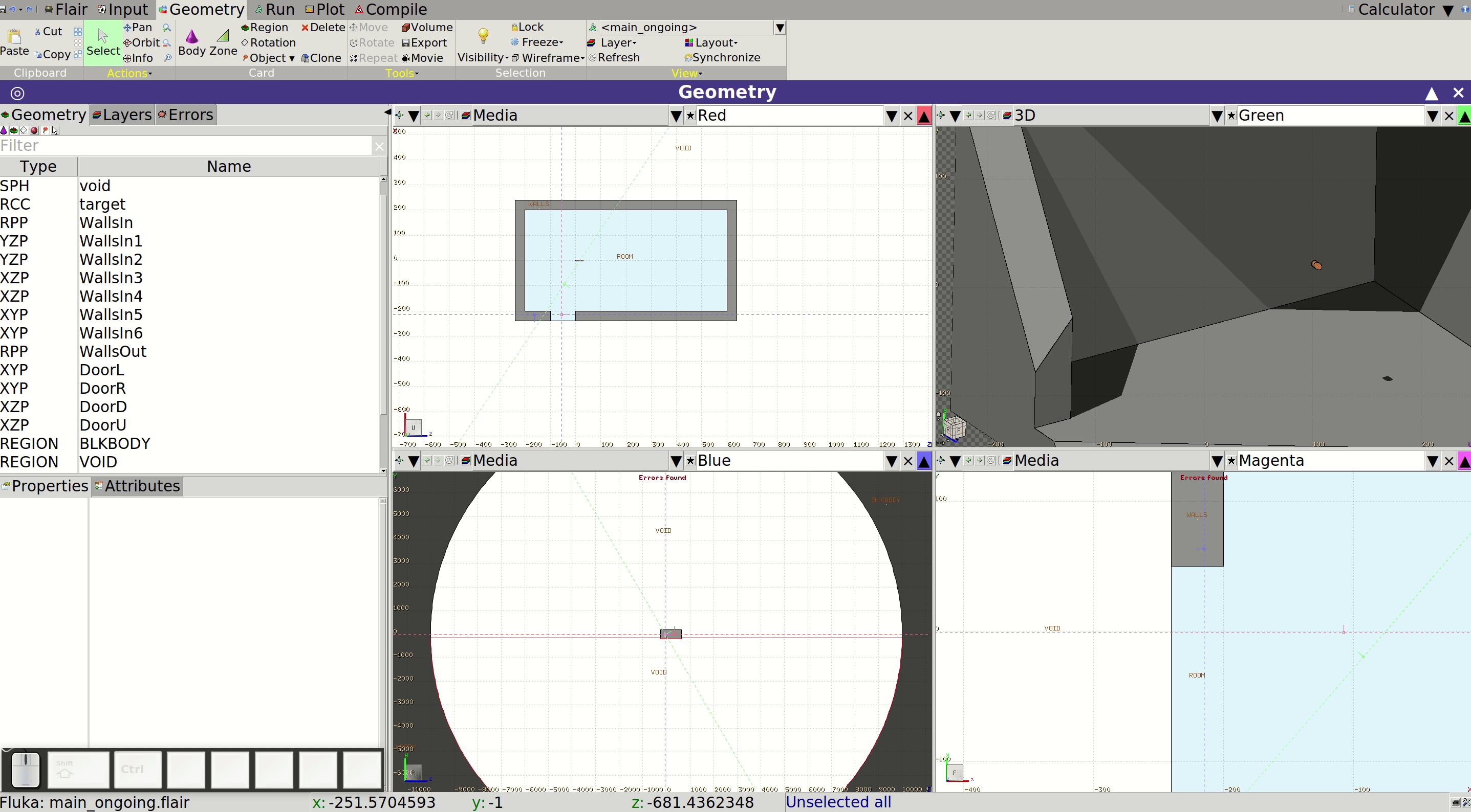
You now have a sound and visually accurate geometry. Take some time to explore it using different viewports, especially 3D. Try selecting the WALLS region and using the Transparency toggle (next to Expand and Optimize) to improve visibility.

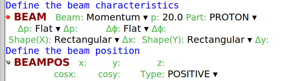
Beam

As discussed earlier, we want to simulate a 20 GeV/c proton beam. We can modify the p and Part entries of the BEAM card accordingly. Since we want a monoenergetic beam, we do not need to specify any momentum spread ($\Delta p$), divergence ($\Delta\phi$), or position spreads ($\Delta x$, $\Delta y$). The default values (zero) are sufficient to model a pencil beam.

The BEAMPOS card, as it stands, provides a beam starting at $x = y = z = 0$ and traveling in the positive $z$ direction. This matches the current position of our target, so no changes are necessary.

Scoring

Next, we will include scoring cards to estimate quantities of interest.

We aim to estimate:

• The particle fluence on the surface of the target
• The energy deposition within the target
• The dose equivalent throughout the room

Let’s begin with the energy deposition in the target. This is important for assessing target integrity under a given irradiation scheme.

To score energy deposition, we’ll use a USRBIN card. Given the cylindrical symmetry of our geometry and beam, an R-$\phi$-Z binning type is ideal. We'll specify a single bin in the $\phi$ dimension, which reduces statistical uncertainty and improves convergence.

Set the particle to ENERGY, and choose unit 21 BIN as the output file. Define the binning as follows:
- 1 mm resolution in $R$
- 2.5 mm resolution in $Z$
- 1 bin in $\phi$

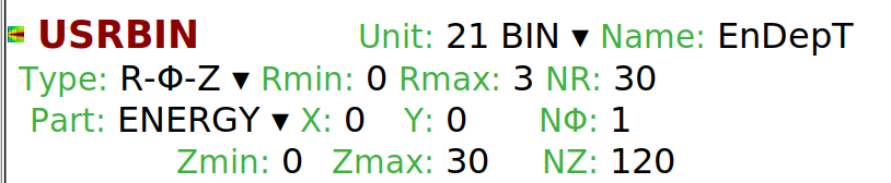
The scoring has been labeled EnDepT.

Now, to assess radiation protection aspects, we’ll estimate the spatial distribution of the dose equivalent in the room. We’ll again use USRBIN, this time with Cartesian X-Y-Z binning. The region will extend beyond the facility walls to observe dose attenuation.

The particle type will be DOSE-EQ. Since we’re more interested in the $X$ and $Z$ variations, we’ll use coarse binning in the $Y$ (height) dimension. Suggested bin sizes are approximately 5 $\times$ 50 $\times$ 5 cm³ ($xyz$):

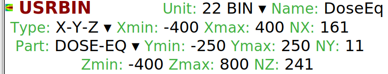
Use unit 22 BIN and name the scoring DoseEq. Note: choosing odd numbers of bins ensures the pencil beam doesn't fall between two bin edges, improving accuracy.

Next, let’s score the particle fluences on the surface of the target using USRBDX, a boundary crossing estimator.

Under the Reg and to Reg fields, set TARGET and ROOM respectively to define the scoring boundary. Leave the Area field empty (default = 1 cm²), and use logarithmic energy binning. Leave the solid angle fields at default values to integrate over $2\pi$.

Create three USRBDX scorings: one each for protons, neutrons, and photons.

• Energy range: [1e-5, 25] GeV for protons and photons
• For neutrons: [1e-12, 25] GeV
• Use 100 bins for each case

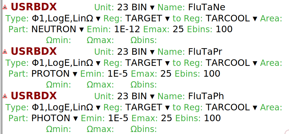
Assign each USRBDX a unique name. All outputs can be written to unit 23 BIN.

Run and process

It’s time to run the simulation.

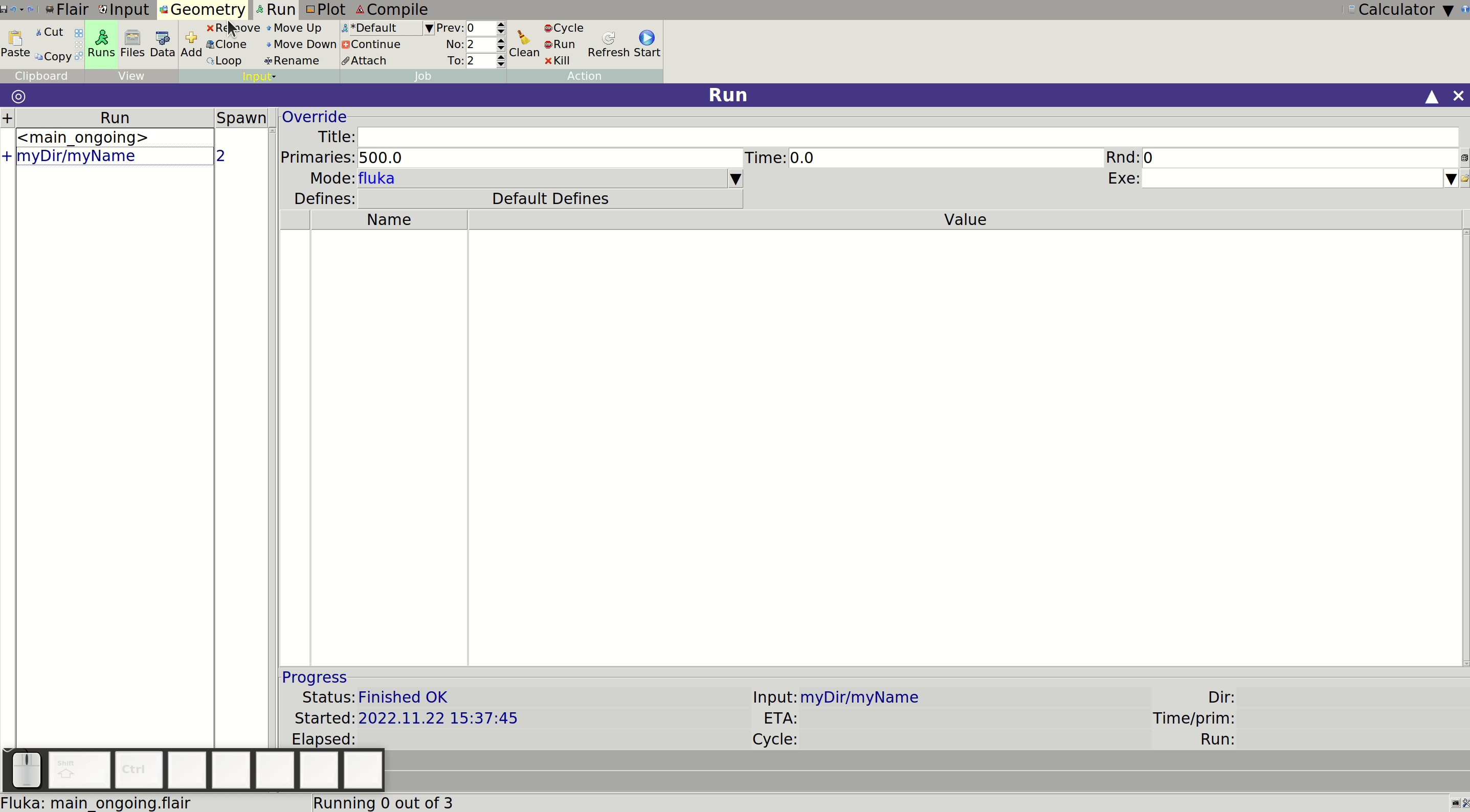
Navigate to the Run tab in Flair. Under the Runs sub-tab, you can configure how the simulation will be executed:

• Number of jobs to run in parallel (spawns)
• Number of cycles
• Number of primary particles per cycle

You may choose a custom name for your run and output directory to organize your files. To configure and launch a run:

• Click the Add button (top-left)
• Enter directory_name/run_name and click Save
• Set spawns (e.g. 2), cycles (e.g. 2), and primaries per cycle (e.g. 500)
• Click Start to launch the simulation

Monitor progress by expanding the run list with the + symbol. You can stop a simulation if it takes too long using STOP Run, adjust parameters, and restart.

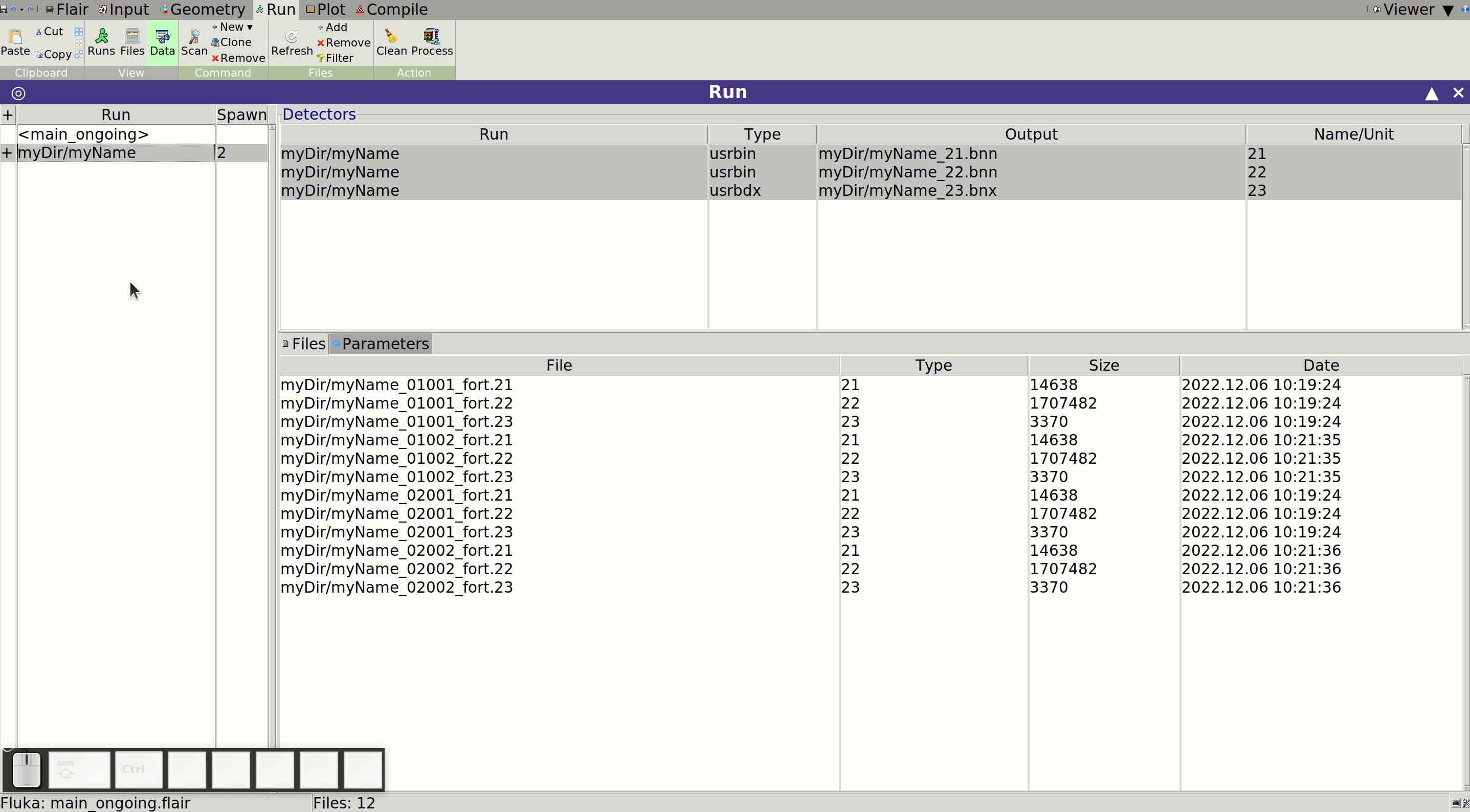
Once finished, process the results:

• Go to the Data sub-tab under Run
• Select your run from the list on the left
• Click Process to merge result files into one per unit

The results are now ready to be plotted and discussed.

Plotting results

Particle fluences

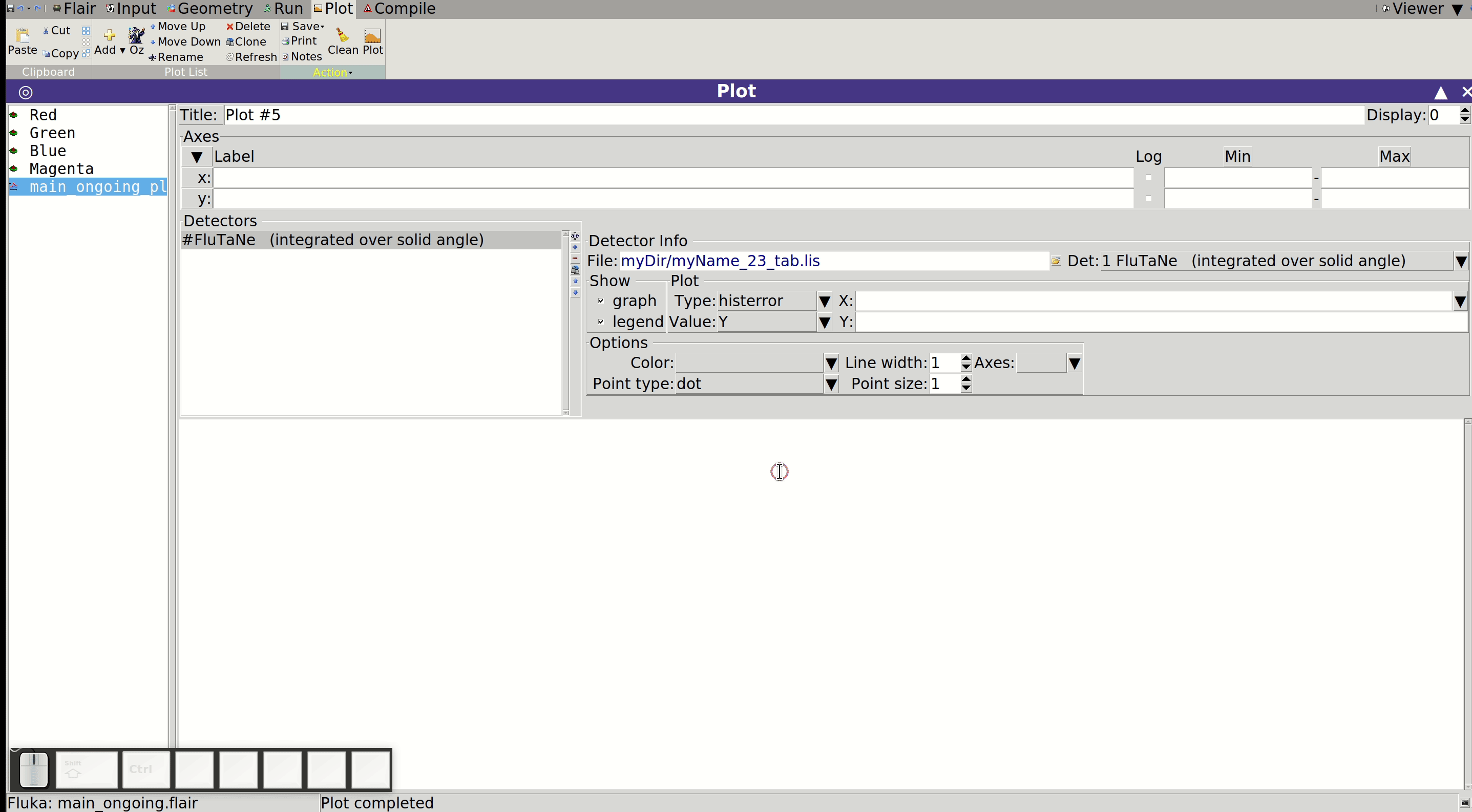
Let us start by plotting the particle fluences resulting from our USRBDX scoring, obtaining the differential spectrum of neutrons, protons and photons crossing the target's surface. To do this:

• Navigate to the Plot tab in Flair.
• Click the Add button (top left)
• Choose USR-1D from the dropdown
• Click the folder icon next to the File field
• Select the file ending in 23_tab.lis. It was created in our "myDir" directory when the simulation results were processed.
• Click Plot

At first, the plot may appear underwhelming—don’t worry! Enable logarithmic scale for both axes by ticking the boxes under the "Log" label. Then add axis labels:
- X-axis: Energy [GeV]
- Y-axis: Fluence [1/cm²/GeV/pr]

To normalize by the scoring surface (i.e., target surface area), input the factor 1/622 or equivalent in the Y: field (FLUKA energy unit is GeV).

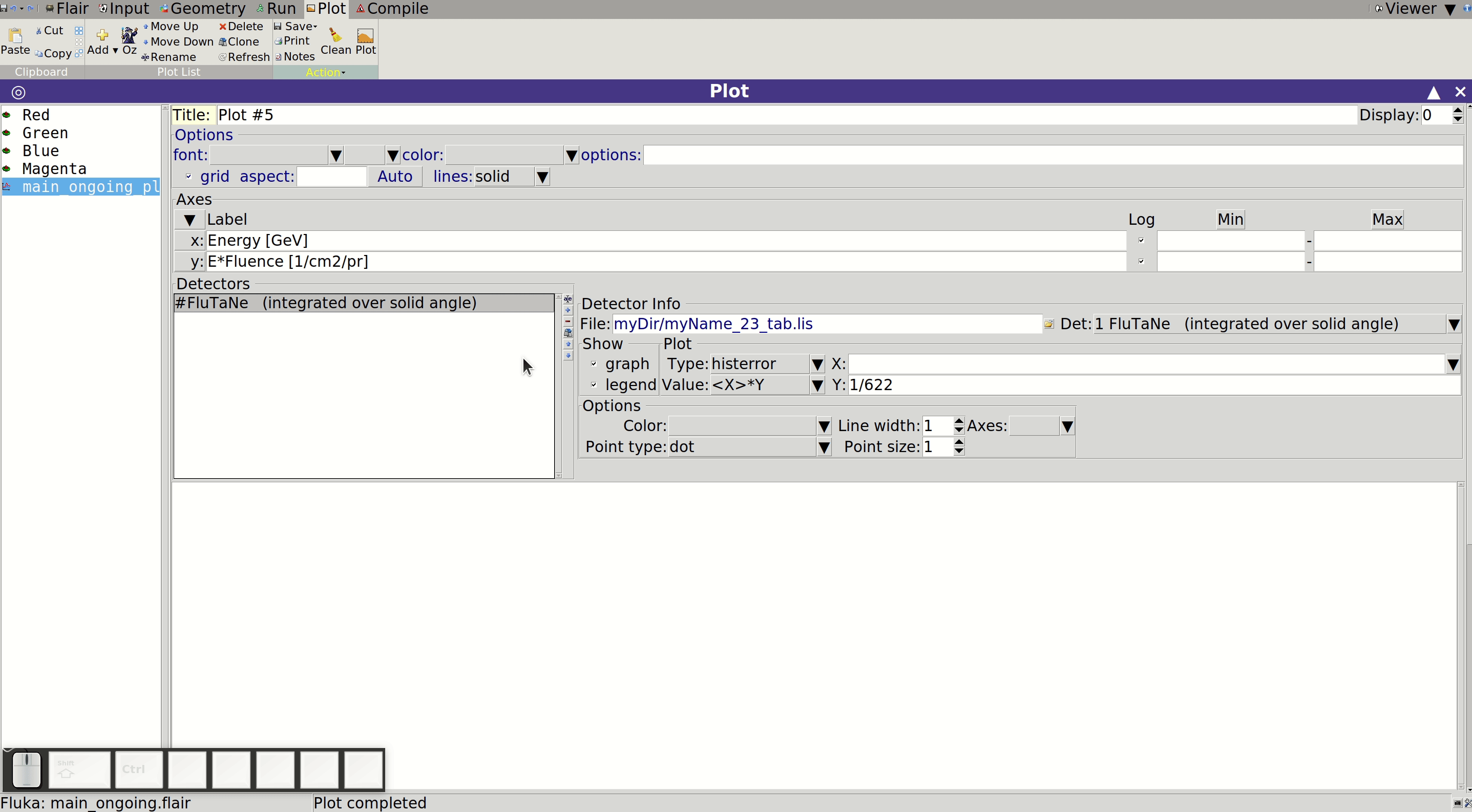
To visualize an iso-lethargic plot (spectrum weighted by energy), change the Value field to < X > * Y. To add a grid, click on Title, then tick the Grid option.

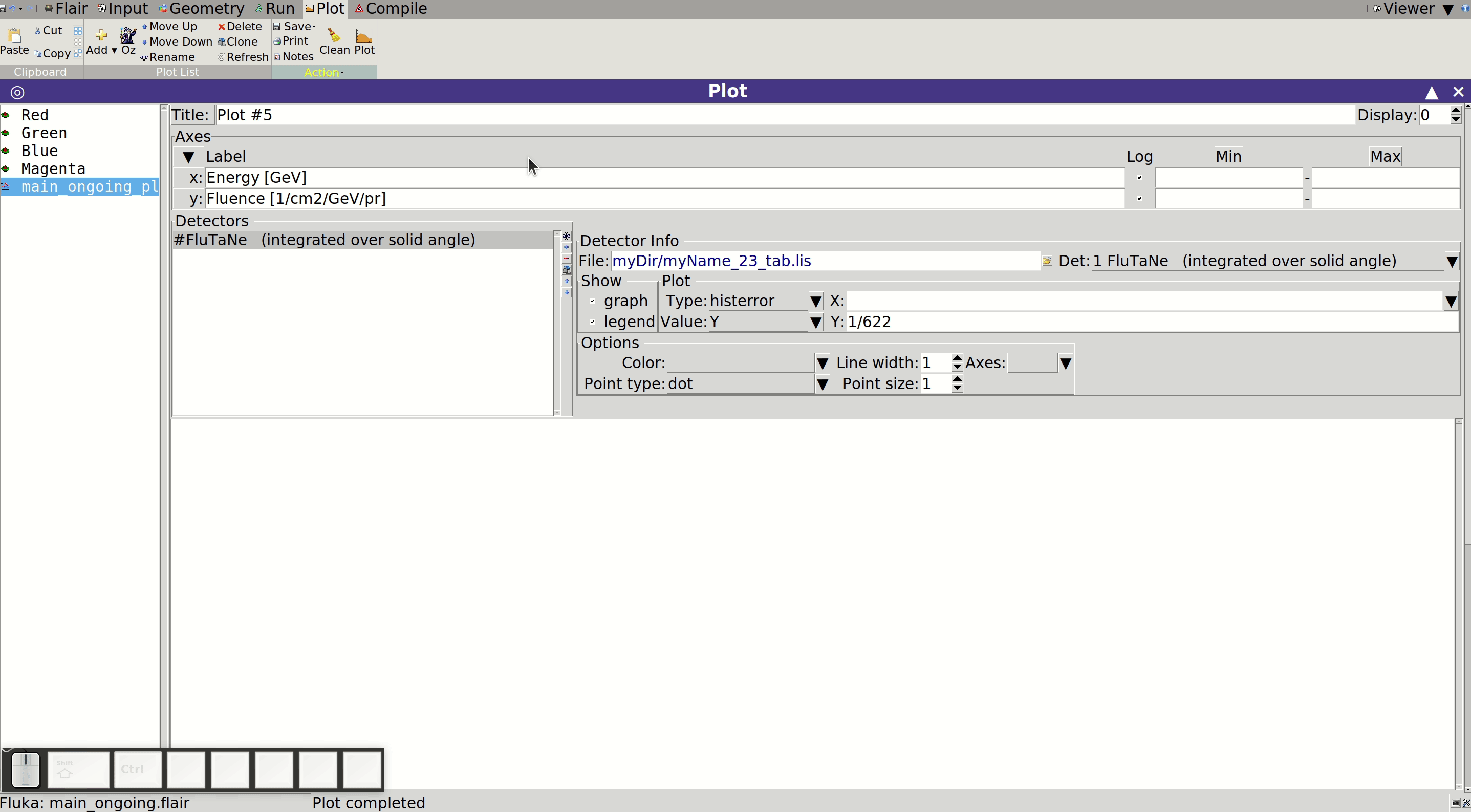
The file name includes 23 because it corresponds to unit 23 BIN, used for all USRBDX cards. Use the Detectors list to choose which one to plot (e.g. protons, neutrons, photons). The second entry for each detector is per steradian; the first is integrated over solid angle.

To add the other two fluence curves:

• Select the existing detector.
• Click the Clone button.
• Change the Det: field to the corresponding entry.
• Assign a distinct color under Options.
• Optionally rename each detector for clarity.

Energy deposition in the target

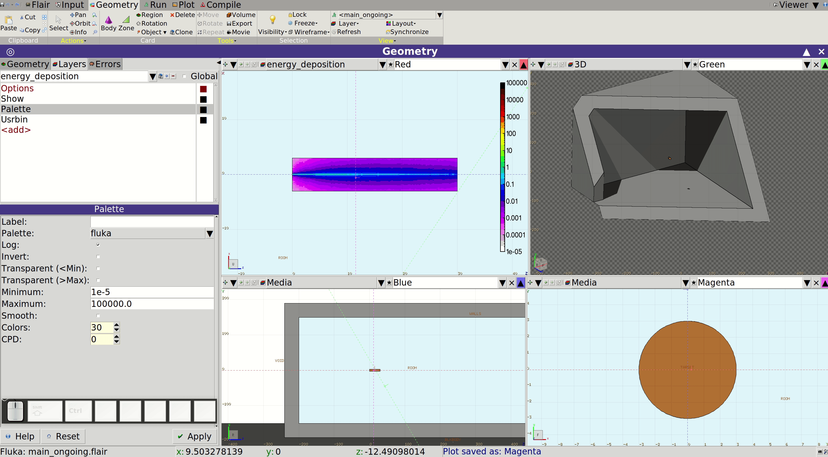
We can plot USRBIN results in Flair using the Plot tab, just as we did for the particle fluences. However, USRBIN data can also be visualized directly in the Geometry tab, overlaid on the geometry itself. This method provides a highly intuitive and visually appealing representation.

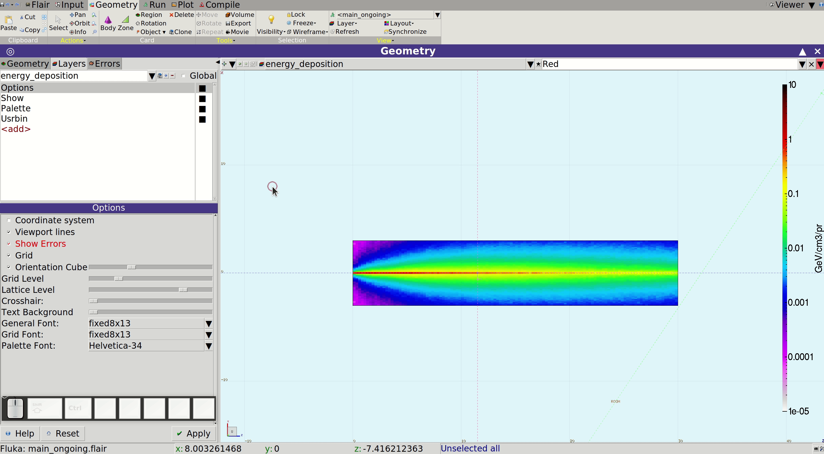
Start by navigating to the Geometry tab and centering a viewport on the target. On the left side of the Flair window, you’ll find three sub-tabs: Geometry, Layers, and Errors. To display USRBIN results on top of the geometry, we need to create a new layer. Click the black down arrow next to the Layers sub-tab to access the default layers. Each viewport displays a selected layer — e.g. Media or 3D, indicated at the top of the viewport.

We’ll now create a new layer to display the USRBIN results for energy deposition in the target:

• Clone the Media layer using the button beside it under Layers.
• Name the new layer something descriptive, like energy_deposition.
• Click and choose Usrbin to add a USRBIN element to the new layer.
• Click the folder icon in the Usrbin menu and select the appropriate result file.

Once added, the new layer can be displayed in any viewport by selecting it.

When a USRBIN is added to a layer, a Palette is automatically created for coloring. You can adjust its minimum, maximum, and other parameters via the new layer's settings. Add a label with appropriate units—GeV/cm³/pr—as defined in USRBIN note 5. Since the bins are regular and their volumes known, FLUKA already includes volume normalization.

To enhance visual continuity, enable the Smooth option to reduce abrupt color changes between adjacent bins. Font sizes for this layer can also be adjusted via the Options menu.

It’s worth familiarizing yourself with the From Input feature in the Usrbin menu. This allows you to preview the spatial extent and granularity of your USRBIN scorings before running a simulation—saving you valuable time when debugging or tuning your setup.

Dose equivalent

Finally, let’s visualize the dose equivalent distribution using the last of our scorings. Just like before, we’ll overlay it on the geometry using the Geometry tab.

Repeat the procedure:

• Create a new layer
• Add a USRBIN item to it
• Load the correct output file

This time, the result units are pSv/pr, as documented in (USRBIN note 9)

Congratulations!
If you’ve successfully followed this example, you now know how to build and run a FLUKA simulation, process the results, and visualize them effectively. Now it's time to carefully review your outputs and ensure they make physical and logical sense.

Welcome to the FLUKA community! Don’t hesitate to reach out via the FLUKA forum if you have questions or need support.